This document provides an overview of wavelet transformation and discrete wavelet transform (DWT). It discusses working with wavelets by convolving signals with wavelet filters and storing the results in coefficients. Properties of wavelets include maximum frequency depending on signal length and recursive partitioning of lowest band. DWT requires an orthonormal wavelet basis and uses scaling functions and wavelets. 2D wavelet transform uses separable transforms with low and high pass filters in each direction. Experimental results show decompositions of images at different levels.

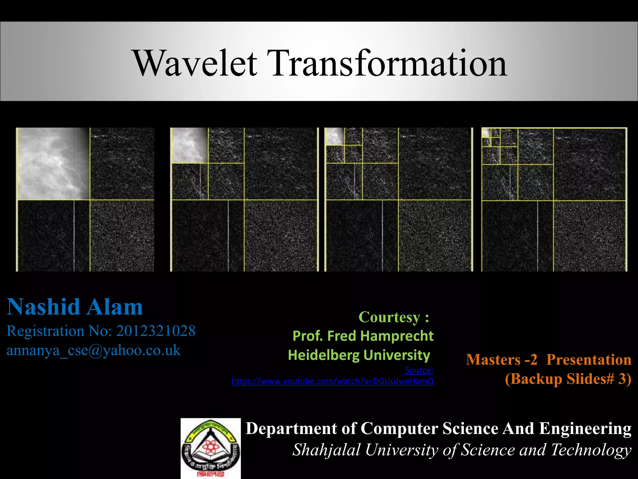
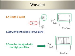
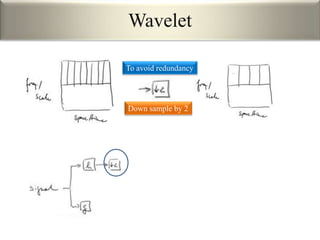
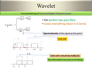
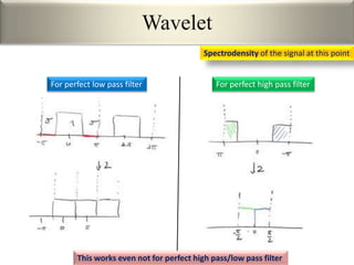
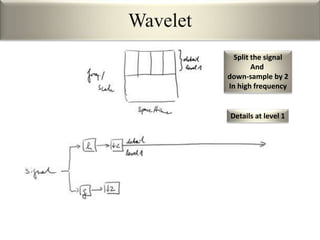
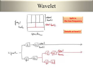
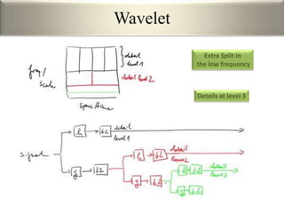
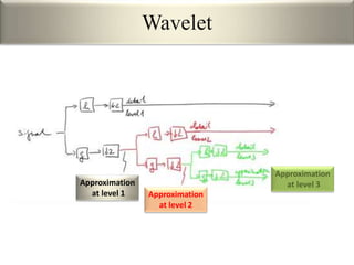
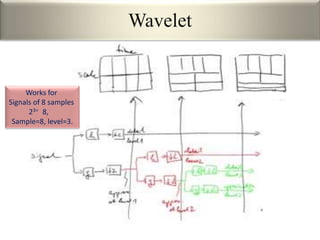
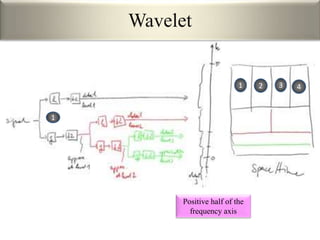
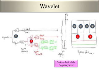
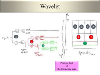
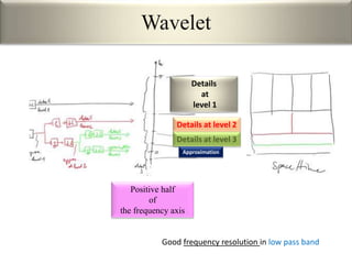
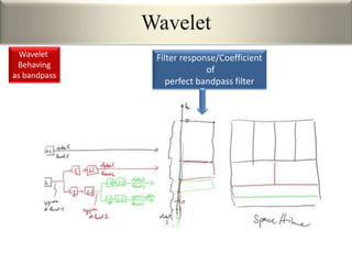
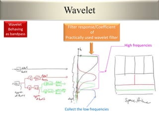
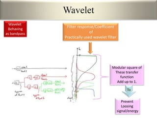
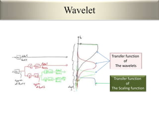
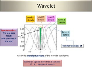
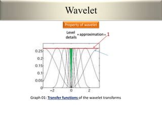
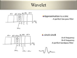
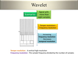
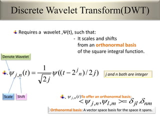
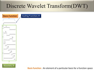
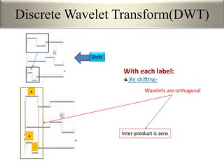
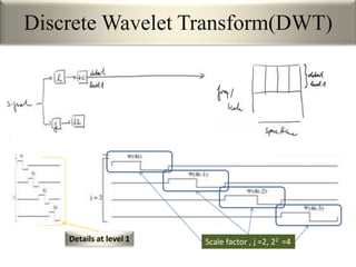
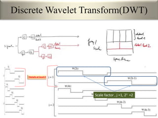
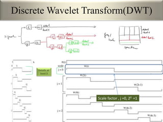
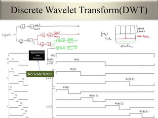
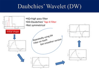
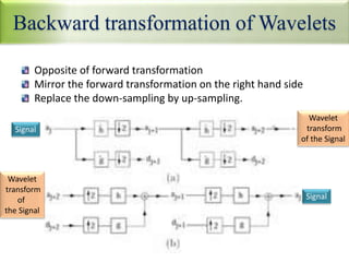
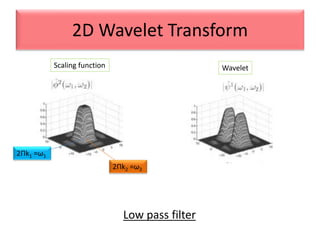
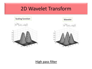
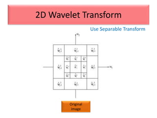
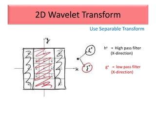
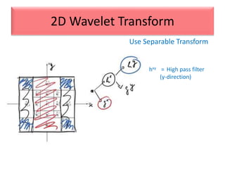
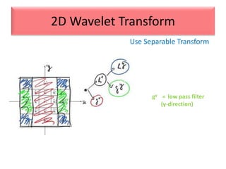
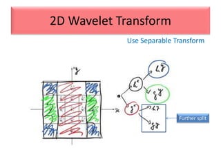
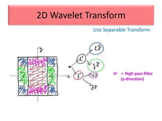
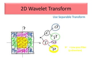
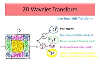
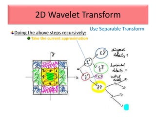
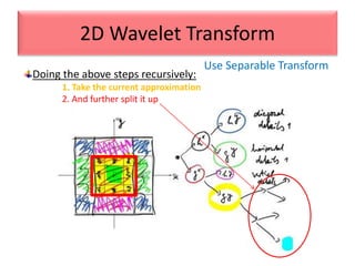
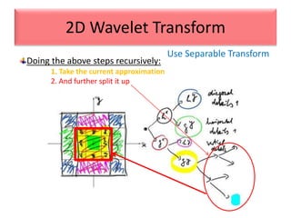
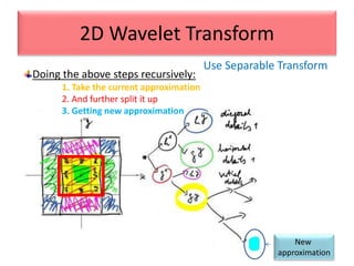
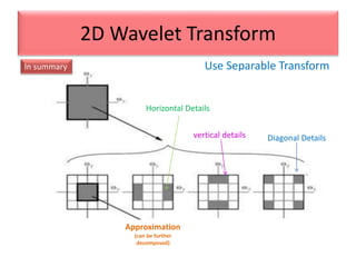
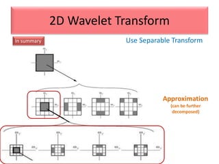
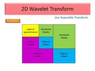
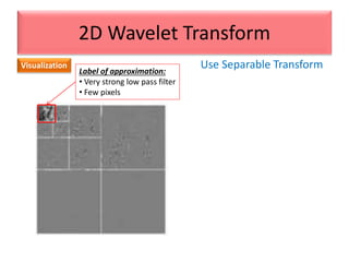
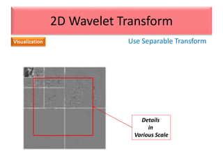
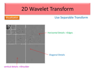
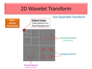
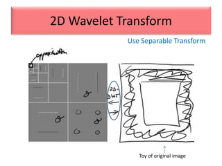
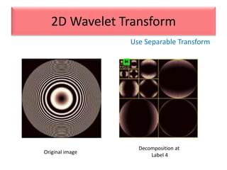
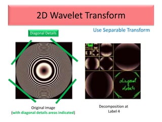
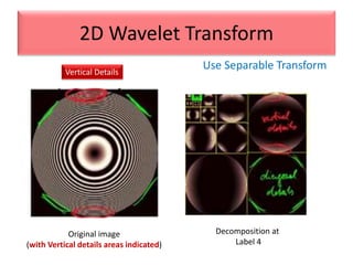
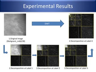
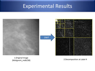
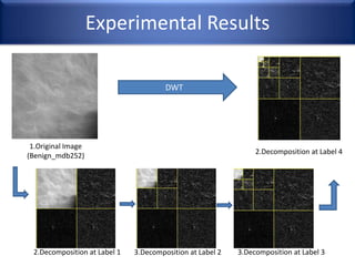
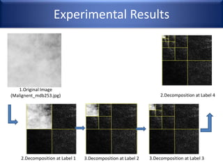
1. Wavelet Transformation
Department of Computer Science And Engineering
Shahjalal University of Science and Technology
Nashid Alam
Registration No: 2012321028
annanya_cse@yahoo.co.uk
Masters -2 Presentation
(Backup Slides# 3)
Courtesy :
Prof. Fred Hamprecht
Heidelberg University
Source:
https://www.youtube.com/watch?v=DGUuJweHamQ

2. Wavelet

3. Wavelet
Working with wavelet:
1. Convolve the signal with wavelet filter(h/g)
2. Store the results in coefficients/frequency response
(Result in number is put in the boxes)
3. Coefficients/frequency response:
- The representation of the signal in the new domain.
Properties:
• Maximum frequency depends on the length of the signal.
• Recursive partitioning of the lowest band in subjective to the application.
Details in upcoming slides

4. Good temper resolution in high frequencies
Good frequency resolution in low pass band
OBTAION:
Wavelet
A high pass filter
Temper resolution : A vertical high-resolution
Frequency resolution : The sample frequency divided by the number of samples
O/P of Low Pass Filter High Pass Filter = A Band Pass Result

5. 1.A length 8 signal
3.Convolve the signal with
the high pass filter
2.Split/divide the signal in two parts
Wavelet

6. To avoid redundancy
Down sample by 2
Wavelet

7. • For perfect low pass filter
• Leave everything intact in 0 (zero)
Spectrodensity of the signal at this point
Unit cell
Unit cell is shrunk by half(1/2)
Wavelet
No information loss due to shrinking
First partitioning of lower and higher frequency band

8. Wavelet
Spectrodensity of the signal at this point
For perfect low pass filter For perfect high pass filter
This works even not for perfect high pass/low pass filter

9. Wavelet
Split the signal
And
down-sample by 2
In high frequency
Details at level 1

10. Wavelet
Split in
the low frequency
Details at level 2

11. Wavelet
Extra Split in
the low frequency
Details at level 3

12. Wavelet
Approximation
at level 3
Approximation
at level 2
Approximation
at level 1

13. Wavelet
Works for
Signals of 8 samples
23= 8,
Sample=8, level=3.

14. Wavelet
Positive half of the
frequency axis
1
1 2 3 4

15. Wavelet
Positive half of the
frequency axis
2
1 21
1 2 3 4

16. Wavelet
Positive half
of
the frequency axis
3
1
2
1 21
1 2 3 4

17. Wavelet
Positive half
of
the frequency axis
Details at level 2
Details at level 3
Details
at
level 1
Approximation
Good frequency resolution in low pass band

18. Wavelet
Filter response/Coefficient
of
perfect bandpass filter
Wavelet
Behaving
as bandpass

19. Wavelet
Filter response/Coefficient
of
Practically used wavelet filter
Collect the low frequencies
High frequencies
Wavelet
Behaving
as bandpass

20. Wavelet
Filter response/Coefficient
of
Practically used wavelet filter
Modular square of
These transfer
function
Add up to 1.
Prevent
Loosing
signal/energy
To
Wavelet
Behaving
as bandpass

21. Code Fragments to do the task
% Extract the level 1 coefficients.
a1 = appcoef2(wc,s,wname,1);
h1 = detcoef2('h',wc,s,1);
v1 = detcoef2('v',wc,s,1);
d1 = detcoef2('d',wc,s,1);
% Display the decomposition up to level 1 only.
ncolors = size(map,1); % Number of colors.
sz = size(X);
cod_a1 = wcodemat(a1,ncolors);
cod_a1 = wkeep(cod_a1, sz/2);
cod_h1 = wcodemat(h1,ncolors);
cod_h1 = wkeep(cod_h1, sz/2);
cod_v1 = wcodemat(v1,ncolors);
cod_v1 = wkeep(cod_v1, sz/2);
cod_d1 = wcodemat(d1,ncolors);
cod_d1 = wkeep(cod_d1, sz/2);
image([cod_a1,cod_h1;cod_v1,cod_d1]);
axis image; set(gca,'XTick',[],'YTick',[]);
title('Single stage decomposition')
colormap(map)
pause
% Here are the reconstructed branches
ra2 = wrcoef2('a',wc,s,wname,2);
rh2 = wrcoef2('h',wc,s,wname,2);
rv2 = wrcoef2('v',wc,s,wname,2);
rd2 = wrcoef2('d',wc,s,wname,2);
Wavelet

22. Wavelet
Transfer function
of
The wavelets
Transfer function
of
The Scaling function

23. Wavelet
Want to understand
The effect of this label
Have to perform
convolution
Understand The effect of each this label

24. Wavelet
Graph 01: Transfer functions of the wavelet transforms
Works for Signals more then 8 samples
23= 8, Sample=8, level=3.
Level 1
details
Level 2
details
Level 3
details
Level 4
details
Level 5
details
Transfer functions of
Approximation:
The low pass
result
That we keep at
the end

25. Wavelet
Graph 01: Transfer functions of the wavelet transforms
Level
details
+approximation= 1
Property of wavelet

26. Wavelet
Approximation is a sinc
- A perfect low pass filter
sincA-sincB
A=A frequency
B=A frequency
-A perfect bandpass filter

27. Wavelet
Signal with
more than
eight samples
Scenario:
Temper resolution : A vertical high-resolution
Frequency resolution : The sample frequency divided by the number of samples
Temper resolution>
Frequency resolution
Increasing
frequency resolution
Decreases
temporal resolution.

28. Discrete Wavelet Transform(DWT)

29. Discrete Wavelet Transform(DWT)
Requires a wavelet ,Ψ(t), such that:
- It scales and shifts
from an orthonormal basis
of the square integral function.
)2/)2((
2
1
)(, jt
j
t n
j
nj  
Scale Shift
Denote Wavelet
j and n both are integer
nmjlmlnj  ., ,, 
To offer an orthonormal basis:)(, tnj
Orthonormal basis: A vector space basis for the space it spans.
.
.

30. Discrete Wavelet Transform(DWT)
Basis Function
Wavelets,Ψ
Basis function : An element of a particular basis for a function space
Scaling Function,Ψ

31. Discrete Wavelet Transform(DWT)
With each label:
By shifting-
+
+
-
Shift
Inter-product is zero
Wavelets are orthogonal

32. Discrete Wavelet Transform(DWT)
Details at level 1 Scale factor , j =2, 22 =4

33. Discrete Wavelet Transform(DWT)
Details at level 2
Scale factor , j =1, 21 =2

34. Discrete Wavelet Transform(DWT)
Details at
level 3
Scale factor , j =0, 20 =1

35. Discrete Wavelet Transform(DWT)
Approximation
Low
frequency
No Scale factor

36. Daubchies’Wavelet (DW)

37. Daubchies’Wavelet (DW)
•H()=high pass filter
•D4=Daubchies’ Tap 4 Filter
•Not symmetrical
Initial shape

39. Backward transformation of Wavelets
Opposite of forward transformation
Mirror the forward transformation on the right hand side
Replace the down-sampling by up-sampling.
Signal
Wavelet
transform
of the Signal
Wavelet
transform
of
the Signal
Signal

40. 2D Wavelet Transform
Scaling function Wavelet
2Πk1 =ω1
2Πk2 =ω2
Low pass filter

41. 2D Wavelet Transform
High pass filter
Scaling function Wavelet

42. Use Separable Transform
2D Wavelet Transform
Original
image

43. hx = High pass filter
(X-direction)
gx = low pass filter
(X-direction)
Use Separable Transform
2D Wavelet Transform

44. hxy = High pass filter
(y-direction)
Use Separable Transform
2D Wavelet Transform

45. gy = low pass filter
(y-direction)
Use Separable Transform
2D Wavelet Transform

46. Use Separable Transform
2D Wavelet Transform
Further split

47. Use Separable Transform
2D Wavelet Transform
hy = High pass filter
(y-direction)

48. Use Separable Transform
2D Wavelet Transform
hy =Low pass filter
(y-direction)

49. Use Separable Transform
2D Wavelet Transform
Four region:
Blue= Diagonal Details at label 1
Green=Horizontal Details at label 1
Purple=vertical details at label 1
Yellow= Approximation at Label 1
(Low pass in both x and y direction)

50. Use Separable Transform
2D Wavelet Transform
Doing the above steps recursively:
Take the current approximation

51. Use Separable Transform
2D Wavelet Transform
Doing the above steps recursively:
1. Take the current approximation
2. And further split it up

52. Use Separable Transform
2D Wavelet Transform
Doing the above steps recursively:
1. Take the current approximation
2. And further split it up

53. Use Separable Transform
2D Wavelet Transform
New
approximation
Doing the above steps recursively:
1. Take the current approximation
2. And further split it up
3. Getting new approximation

54. Use Separable Transform
2D Wavelet Transform
Diagonal Details
Horizontal Details
vertical details
Approximation
(can be further
decomposed)
In summary

55. Use Separable Transform
2D Wavelet Transform
In summary
Approximation
(can be further
decomposed)

56. Use Separable Transform
2D Wavelet Transform
Visualization
Label of
approximation
Horizontal
Details
Horizontal
Details
Vertical
Details
Diagonal
Details
Vertical
Details
Diagonal
Details

57. Use Separable Transform
2D Wavelet Transform
Visualization
Label of approximation:
• Very strong low pass filter
• Few pixels

58. Use Separable Transform
2D Wavelet Transform
Visualization
Details
in
Various Scale

59. Use Separable Transform
2D Wavelet Transform
Visualization
vertical details ->Shoulder
Horizontal Details ->Edges
Diagonal Details

60. Use Separable Transform
2D Wavelet Transform
More
precise
Visualization
Original image:
Gray square on a
Black Background
Diagonal Details
Horizontal Details
(row by row)
Vertical details
(column by column)

61. Use Separable Transform
2D Wavelet Transform
Toy of original image

62. Use Separable Transform
2D Wavelet Transform
Decomposition at
Label 4
Original image

63. Use Separable Transform
2D Wavelet Transform
Decomposition at
Label 4
Original image
(with diagonal details areas indicated)
Diagonal Details

64. Use Separable Transform
2D Wavelet Transform
Vertical Details
Decomposition at
Label 4
Original image
(with Vertical details areas indicated)

65. Experimental Results

66. Experimental Results
DWT
1.Original Image
(Malignent_mdb238) 2.Decomposition at Label 4
2.Decomposition at Label 1 3.Decomposition at Label 2 3.Decomposition at Label 3

67. Experimental Results
DWT
1.Original Image
(Malignent_mdb238) 2.Decomposition at Label 4

68. Experimental Results
1.Original Image
(Benign_mdb252)
2.Decomposition at Label 4
2.Decomposition at Label 1 3.Decomposition at Label 2 3.Decomposition at Label 3
DWT

69. Experimental Results
1.Original Image
(Malignent_mdb253.jpg) 2.Decomposition at Label 4
2.Decomposition at Label 1 3.Decomposition at Label 2 3.Decomposition at Label 3

70. CT vs. DWT
DWT Target Goal:
1.Applying a DWT to decompose a digital mammogram into different subbands.
2.The low-pass wavelet band is removed (set to zero) and
the remaining coefficients are enhanced.
3.The inverse wavelet transform is applied to recover
the enhanced mammogram containing microcalcifications [7].
7. Wang T. C and Karayiannis N. B.: Detection of Microcalcifications in Digital Mammograms Using Wavelets, IEEE
Transaction on Medical Imaging, vol. 17, no. 4, (1989) pp. 498-509
The results obtained by the Contourlet Transformation (CT)
are compared with
The well-known method based on the discrete wavelet transform