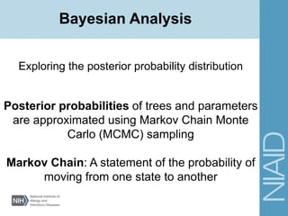
Kurt Wollenberg, PhD
Phylogenetics Specialist
Bioinformatics and Computational Biology Branch (BCBB)
Office of Cyber Infrastructure and Computational Biology
Virus Sequence Alignment and
Phylogenetics
21 June 2019
We Are BCBB!
2
 Group of (so far) 52
• Bioinformatics Software Developers
• Computational Biologists
• Project Management & Analysis Professionals
The Goal
3
Data
Phylogenetics
Software
Tree
Data
Phylogenetics
Software Tree
Why analyze
biological
sequences?
4
Biological sequences
• DNA contains the information basic to every process in a
cell
• Proteins (and RNA) are the machines performing cellular
processes
• Passed from one generation to the next
5
Sequence data are genealogical
6
Why analyze sequences
using comparative
methods?
7
Comparative Methods
Comparative Methods
• Sequences related by common ancestry
• Analyzing samples with the trait against those
without it
• The Grail: Finding nucleotide X at site Y in gene
Z which correlates with the presence of the trait
• Correlation vs causation
8
Hierarchy of Life
• Carl Linnaeus (1707 - 1778)
• Swedish physician/naturalist
• Hierarchical organization of life
• Binomial system of scientific names
10
Common Ancestry
• Charles Darwin (1809 - 1882)
• Artificial selection: crops and livestock
• Fossil record: change over time
• Biogeography: similarities across regions and
differences within locales
• Descent with modification ➯ continuity of life
• Natural selection: change in population traits due to
individual interactions with their environment
11
Common Ancestry
12
“… I believe this element of descent is the
hidden bond of connexion which naturalists
have sought under the term of the Natural
System” p. 433
“Naturalists try to arrange the species, genera,
and families in each class, on what is called the
Natural System. But what is meant by this
system?” p.413
What’s so special about viruses?
• Short generation time
• Rapid evolution
• Genotypes - easy, phenotypes - hard
• Large populations
• Structured populations
• Rigorous temporal sampling of genotypes
• Shorter genomes → more WGS data
14
and BLAST: Basic Local Alignment Search Tool
• Sequence Alignment: Assigning homology to
sites among a group of known sequences
• BLAST: Alignment of one sequence with many
unknown sequences
PAIRWISE ALIGNMENT
HOMOLOGY vs. ANALOGY
15
common ancestry convergence
16
• Sequence Alignment: Assigning homology to
sites among a group of known sequences
• Alignment of single loci
o Clustal(W,X,Omega), MUSCLE, TCoffee, MAFFT
• Alignment of overlapping contigs
o Sequencher, Lasergene
• Alignment of short reads
o BWA, Bowtie, SOAP, MAQ
PAIRWISE ALIGNMENT
17
• Single locus
PAIRWISE ALIGNMENT
>GeneA_Human
ATGGGCCTTATATGCGTGATGCTGAAAG
>GeneA_Gorilla
ATGGGACTTATCTGCGTGATGCTGACAG
>GeneA_Macaque
ATGGGTCTCATATGTGTGATGCTTACAG
>GeneA_Mouse
ATGGCCCTGATATGCGTGATGCTGAACG
>GeneA_Sheep
ATGGCCCTAATATGC---AGGCTGAACG
18
• Overlapping contigs
PAIRWISE ALIGNMENT
ATGGGCCTTATATGCGTGATGCTGAAAG
TTATATGCGTGATGCTGAAAGGGCTTAG
ATATGCGTGATGCTGAAAGGGCTTAGAAAT
TGCGTGATGCTGAAAGGGCTTAGAAATT
ATGCTGAAAGGGCTTAGAAATTCGG
AAAGGGCTTAGAAATTGCGGCTAGGCCTCC
CGGCTAGGCCTCCGAACGC
TACCCGGAATATACGCACTA
CACTACGACTTTCCCGAATCTTTAAGCC
CTTTCCCGAATCTTTAAGCCGATCCGGA
19
• Short reads
PAIRWISE ALIGNMENT
HBA_HUMAN GSAQVKGHGKKVADALTNAVAHVDDMPNALSALSDLHAHKL
G+ +VK+HGKKV A+++++AH+D++ +++++LS+LH KL
HBB_HUMAN GNPKVKAHGKKVLGAFSDGLAHLDNLKGTFATLSELHCDKL
HBA_HUMAN GSAQVKGHGKKVADALTNAVAHV---D--DMPNALSALSDLHAHKL
++ ++++H+ KV + +A ++ +L+ L+++H+ K
LGB2_LUPLU NNPELQAHAGKVFKLVYEAAIQLQVTGVVVTDATLKNLGSVHVSKG
HBA_HUMAN GSAQVKGHGKKVADALTNAVAHVDDMPNALSALSD----LHAHKL
GS+ + G + +D L ++ H+ D+ A +AL D ++AH+
F11G11.2 GSGYLVGDSLTFVDLL--VAQHTADLLAANAALLDEFPQFKAHQE
20
PAIRWISE ALIGNMENT
μt = 0.25
A C G T
A 0.5259 0.1580 0.1580 0.1580
C 0.1580 0.5259 0.1580 0.1580
G 0.1580 0.1580 0.5259 0.1580
T 0.1580 0.1580 0.1580 0.5259
21
PAIRWISE ALIGNMENT
Jukes-Cantor Substitution Probabilities
Jukes-Cantor
(One substitution type, equal nucleotide frequencies)
Independent nucl. freq. Two substitution types .
F81/TN82 Kimura 2-Parameter (K2P)
Two substitution types Indep. nucl. freq. Three substitution types .
HKY85/F84 Kimura 3 subst. type (K3ST)
Three substitution types Six substitution types .
Tamura-Nei (TrN) Symmetric (SYM)
Six substitution types Independent nucl. freq. .
General time-reversible (GTR)
Substitution Models
Protein Score Matrices
Similarity of Amino Acids
23
From Esquivel RO, et al.. 2013. Advances in Quantum Mechanics, Chapter 27 InTech.
PAIRWISE ALIGNMENT
Protein Score Matrices
• Derived from empirical data
• Account for depth of relationship among the data
• Expressed as log-odds ratio:
- Logarithm of the ratio of the probabilities of two
residues being aligned due to homology versus
random chance
24
PAIRWISE ALIGNMENT
Protein Substitution Matrices
• PAM250: Based on phylogenies where all sequences
differ by no more than 15%.
• BLOSUM62: Based on clusters of sequences with
greater than 62% identical residues.
PAIRWISE ALIGNMENT
25
WYFVLIMKRHQEDNGAPTSC
W
Y
F
V
L
I
M
K
R
H
Q
E
D
N
G
A
P
T
S
C
112132313322344234232
7311112221232323222
610003313333324222
41312332233302021
4222232343413121
413333333413121
51120232312121
5211110211103
501020212113
80011222213
5200211103
520211104
61121103
6022013
602203
41010
7113
511
41
9
-----------------
----------------
--------------
-----------
-------------
-------------
------------
-------
-------
-------
-----
-----
-----
---
---
-
---
-
-
BLOSUM62
26
Protein Substitution Matrices
Multiple Sequence Alignment
• Global alignment (Needleman-Wunsch)
• Assign homology across the entire sequence
• Clustal
• Local alignment (Smith-Waterman)
• Assign homology for subsequences
• MUSCLE and BLAST
• Good for aligning very divergent sequences
• Inspect and edit your alignment!
Multiple Sequence Alignment
28
The Progressive Alignment Algorithm
Unaligned
Sequences
Distance
Matrix
Aligned Sequences
MSA1
Kimura Distance
Matrix
Aligned Sequences
MSA2
Subtree Alignment
Profiles
Align Subtree Profiles
MSAsp
Better!
Not Better
From RC Edgar 2004, NAR 32: 1792-1797
UPGMA tree
UPGMA tree 2Delete edge from UPGMA
tree 2
Multiple Sequence Alignment
MSA with MEGA7
Multiple Sequence Alignment
MSA with MEGA7
NEVER
directly input the output of a MSA program into an
analysis program!
ALWAYS
inspect the alignment to improve it.
Multiple Sequence Alignment
31
Multiple Sequence Alignment
• Clustal
• Your own computer
• Web Server
• NIAID HPC cluster
• MUSCLE
• Your own computer
• Web Server
• NIAID HPC cluster
• MAFFT
• Web Server
Programs
34
Multiple Sequence Alignment
Multiple Sequence Alignment Editors
• Geneious
• MacVector
• MegAlign (Lasergene)
Multiple Sequence Alignment
35
Commercial Software Public Domain Software
• AliView
• GeneDoc
• BioEdit
ClustalW
http://www.clustal.org/
Muscle
http://www.drive5.com/muscle/download3.6.html
MAFFT
http://mafft.cbrc.jp/alignment/server/
MEGA7
https://www.megasoftware.net/
AliView
http://www.ormbunkar.se/aliview/
GeneDoc
http://genedoc.software.informer.com/
BioEdit
http://www.mbio.ncsu.edu/BioEdit/bioedit.html
Web Resources
36
What’s next?
After the break
Building trees with our MSA
What is a phylogenetic tree?
• Reconstruction of biological history
• Based on similarities and differences among
homologous attributes (characters) of the entities
under scrutiny
• Molecular characters (sequences, usually) are
most often found only in extant organisms
A
D
E
C
B
Internal branches
Terminal branches
Tips
or
leaves Nodes
What is a phylogenetic tree?
Unrooted Rooted
What is a phylogenetic tree?
Two approaches to tree building
•Application of an algorithm to build the best tree from
the data
•Evaluation of multiple possible best trees using an
optimality criterion
The algorithm approach:
Distance Methods
• Distance calculated based on a specific
substitution model (J-C, Kimura, BLOSUM64, etc.)
• Distances from each sequence to all others are
calculated and stored in a matrix
• Tree then calculated from the distance matrix using
a specific tree-building algorithm
μt = 0.25
A C G T
A 0.5259 0.1580 0.1580 0.1580
C 0.1580 0.5259 0.1580 0.1580
G 0.1580 0.1580 0.5259 0.1580
T 0.1580 0.1580 0.1580 0.5259
43
SUBSTITUTION MODEL
Jukes-Cantor Substitution Probabilities
WYFVLIMKRHQEDNGAPTSC
W
Y
F
V
L
I
M
K
R
H
Q
E
D
N
G
A
P
T
S
C
112132313322344234232
7311112221232323222
610003313333324222
41312332233302021
4222232343413121
413333333413121
51120232312121
5211110211103
501020212113
80011222213
5200211103
520211104
61121103
6022013
602203
41010
7113
511
41
9
-----------------
----------------
--------------
-----------
-------------
-------------
------------
-------
-------
-------
-----
-----
-----
---
---
-
---
-
-
BLOSUM62
44
SUBSTITUTION MODEL
Tree-Building Algorithms
• UPGMA
• Neighbor-Joining
The algorithm approach:
Distance Methods
The algorithm approach:
Neighbor-joining Calculation
Hillis, Moritz, and Mable 1996, p. 489
A to Node 1 distance = (0.2147 + 0.3091 - 0.2795)/2 = 0.1222
B to Node 1 distance = (0.2991 + 0.3399 - 0.2795)/2 = 0.1798
E to Node 1 distance = (0.3943 + 0.4298 - 0.2795)/2 = 0.2719
C to Node 1 distance = 0.2795/2 + (1.1876 - 1.3574)/6 = 0.1114
D to Node 1 distance = 0.2795 - 0.1114 = 0.1681
R
0.9279
1.0163
1.1876
1.3574
1.2616
A B C D E
A - 0.1715 0.2147 0.3091 0.2326
B - 0.2991 0.3399 0.2058
C - 0.2795 0.3943
D - 0.4289
E -
-0.4766
-0.4905 -0.4356
-0.4527 -0.4514 -0.5689
-0.4972 -0.5535 -0.4221 -0.4441
The algorithm approach:
Neighbor-joining Calculation
Hillis, Moritz, and Mable 1996, p. 489
B to Node 2 distance = (0.1715 + 0.1798 - 0.1222)/2 = 0.1146
E to Node 2 distance = (0.2326 + 0.2719 - 0.1222)/2 = 0.1912
A to Node 2 distance = 0.1222/2 + (0.5263 – 0.5739)/4 = 0.0492
Node 1 to Node 2 distance = 0.1222 – 0.0492 = 0.0730
R
0.5263
0.5571
0.7103
0.5739
A B E Node 1
A - 0.1715 0.2326 0.1222
B - 0.2058 0.1798
E - 0.2719
Node 1 -
-0.3701
-0.3856 -0.4278
-0.4278 -0.3856 -0.3701
The algorithm approach:
Neighbor-joining Calculation
Hillis, Moritz, and Mable 1996, p. 489
E to Node 3 distance = (0.2058 0.1912 - 0.1146)/2 = 0.1412
B to Node 3 distance = 0.1146/2 + (0.3204 – 0.3058)/2 = 0.0646
Node 2 to Node 3 distance = 0.1146 – 0.0646 = 0.0500
R
0.3204
0.3970
0.3058
B E Node 2
B - 0.2058 0.1146
E - 0.1912
Node 2 -
-0.5116
-0.5116 -0.5116
The algorithm approach:
Neighbor-joining Calculation
A B
C
D
E
0.141
0.065
0.050
0.049
0.073
0.168
0.111
Phylogeny Construction: Neighbor-Joining
MEGA7
Phylogeny Construction: Neighbor-Joining
MEGA7
Phylogeny Construction: Neighbor-Joining
MEGA7
Phylogeny Construction: Neighbor-Joining
MEGA7
Phylogeny Construction: Neighbor-Joining
MEGA7
The optimality criterion approach
• Build a tree or trees
• Evaluate the tree(s) using a specific numerical
optimality criterion
• Most common optimality criteria
• Maximum parsimony
• Maximum likelihood
• Explore tree space to find the optimal tree
Occam’s Razor: The simplest explanation is
the preferred explanation.
The tree requiring the minimal number of
changes is the optimal tree.
A step is any change in the data from one state
to another
Optimality Criterion: Parsimony
• Build the initial tree
• Construct a neighbor-joining tree
• Stepwise addition
• Calculate the tree score
• Count steps (parsimony)
• Calculate likelihood of the data given the tree
• Explore tree space
• Branch swapping
• Tree bisection and reconnection (TBR)
• Is this the best tree? (Stopping criteria)
The optimality criterion approach
•Stepwise addition
•Choose three taxa and join
•Random, or closest
•Select a new taxon to add
•Calculate the optimal 4-taxa tree
•Repeat until all taxa are joined
Building the initial tree
The optimality criterion approach
Building the initial tree
BC
D
G
C
D
G
A
B
C D
E
F
G
B
The optimality criterion approach
•Nearest neighbor interchange
•Subtree pruning and regrafting
•Tree bisection and reconnection
Exploring tree space: Branch swapping
The optimality criterion approach
Branch swapping: Tree bisection and
reconnection
A
B
C D
E
F
G
X
C
A
B D
E
F
G
A
C
B G
F
D
E
The optimality criterion approach
Beware! Hill climbing can often
lead to local maxima rather than
a global solution.
Exploring tree space
The optimality criterion approach
Exploring tree space
The optimality criterion approach
Counting changes (Fitch parsimony)
Is this tree optimal?
The tree The data
S1: AAG
S2: AAA
S3: GGA
S4: AGA
The optimality criterion approach
Counting changes (Fitch parsimony)
Is this tree optimal?
The tree The data
S1: A
S2: A
S3: G
S4: A
{A}  {A} = {A}
0 step
{A}  {AG} = {A}
0 step
{A}  {G} = Ø
{A} U {G} = {AG}
1 step
Position 1
The optimality criterion approach
Counting changes (Fitch parsimony)
Is this tree optimal?
The tree The data
S1: A
S2: A
S3: G
S4: G
{A}  {A} = {A}
0 step
{A} U {G} = {AG}
1 step
{G}  {G} = {G}
0 step
Position 2
The optimality criterion approach
Counting changes (Fitch parsimony)
Is this tree optimal?
The tree The data
S1: A
S2: G
S3: A
S4: A
{A} U {G} = {AG}
1 step
{AG}  {A} = {A}
0 step
{A}  {A} = {A}
0 step
Position 3
The optimality criterion approach
Counting changes (Fitch parsimony)
Is this tree optimal?
The tree The data
S1: AAG
S2: AAA
S3: GGA
S4: AGA
Total
steps:
3
The optimality criterion approach
Counting changes (Fitch parsimony)
Is this tree optimal?
The tree The data
S1: AAG
S3: GGA
S2: AAA
S4: AGA
Total
steps:
4
The optimality criterion approach
Counting changes (Fitch parsimony)
Is this tree optimal?
The tree The data
S1: AAG
S4: AGA
S2: AAA
S3: GGA
Total
steps:
4
The optimality criterion approach
Counting changes (Fitch parsimony)
Is this tree optimal?
The tree The data
S1: AAG
S2: AAA
S3: GGA
S4: AGA
Optimal
Tree!
Total
steps:
3
The optimality criterion approach
Optimality Criterion: Likelihood
Calculating likelihood
The DataThe Tree
S1: AAG
S2: AAA
S3: GGA
S4: AGA
L(Tree) = Prob(Data|Tree) = ∏iProb(Data(i)|Tree)
Calculating likelihood: Setting parameters
What values do you use for the substitution model?
Run jModelTest (or ProtTest for protein MSAs)
Optimality Criterion: Likelihood
L(Tree) = Prob(Data|Tree) = ∏iProb(Data(i)|Tree)
Calculating likelihood: jModelTest
Optimality Criterion: Likelihood
Calculating likelihood: jModelTest
Calculating likelihood: jModelTest Results
Optimality Criterion: Likelihood
Substitution models
http://www.molecularevolution.org/resources/models/nucleotide
Calculating likelihood: jModelTest Results
Optimality Criterion: Likelihood
Substitution models
http://www.molecularevolution.org/resources/models/nucleotide
Calculating likelihood: jModelTest Results
Optimality Criterion: Likelihood
Calculating likelihood: MEGA7 Options
Optimality Criterion: Likelihood
Substitution models
http://www.molecularevolution.org/resources/models/nucleotide
Calculating likelihood: MEGA7 Results
Optimality Criterion: Likelihood
The Gamma Distribution
Mean = kθ Shape parameter = θ
Coefficient of Variation = 1/√θ
How reliable are my trees?
Bootstrapping (nonparametric)
Bootstrapping
the ideal world
Build replicates by resampling from unlimited data
All the data in
the world
Sample n
Sample 3
Sample 2
Sample 1 Tree 1
Tree 2
Tree 3
Tree n
Estimate
of the
true
phylogeny
Build pseudoreplicates of unlimited data by
sampling with replacement from limited data
Limited
data
The Sample
Tree 1
Tree 2
Tree 3
Tree n
Estimate of
the
variance of
the true
phylogeny
Ψsample n
Ψsample 3
Ψsample 2
Ψsample 1
Tree
Estimate of the
true phylogeny
Bootstrapping
the real world
Calculating likelihood: Programs
PAUP* – Commercial, NIH Biowulf, or NIAID HPC
DNA only
PHYLIP – Download, NIH Biowulf, or NIAID HPC
dnaml and proml programs
MEGA – Download for free from www.megasoftware.net
PAML – Download, NIH Biowulf, or NIAID HPC
RaxML – Download or NIH BioWulf or webserver
PhyML – Download or NIAID HPC or webserver
GARLi – Download or NIAID HPC or webserver
Generally the user has more flexibility with a local program.
But local programs can hog your computer.
FASTA
Input File Formats
>MC1_01B4fs
TGCACTAATAATCTGATT---------AATATCACTGAGAATACTAATAATACCATTACT
>MC1_01A10
TGCACT---AATCTGACAAAGGCTATTAAGACCAATGGGAATGCTAATAATACCAGTACT
>MC1_01C1
TGCACTAATAATCTGATT---------AATATCACTGAGAATACTAATAATACCATTACT
>MC1_01A20
TGCACTAATAATCTGACAAAGGCTAGTAATGCCACTGAGAAGGCTAATAATACCATTACT
>MC1_01TA1
TGCACTAATAATCTGATT---------AATATCACTGAGAATACTAATAATACCATTACT
Phylogenetics program input file formats
PHYLIP
1st line: Number of sequences(space)Number of sites
2nd line: Sequence ID (10 characters max) Sequence
Input File Formats
Phylogenetics program input file formats
5 60
MC1_01B4fsTGCACTAATAATCTGATT---------AATATCACTGAGAATACTAATAATACCATTACT
MC1_01A10 TGCACT---AATCTGACAAAGGCTATTAAGACCAATGGGAATGCTAATAATACCAGTACT
MC1_01C1 TGCACTAATAATCTGATT---------AATATCACTGAGAATACTAATAATACCATTACT
MC1_01A20 TGCACTAATAATCTGACAAAGGCTAGTAATGCCACTGAGAAGGCTAATAATACCATTACT
MC1_01TA1 TGCACTAATAATCTGATT---------AATATCACTGAGAATACTAATAATACCATTACT
NEXUS
#NEXUS
begin data;
dimensions ntax=9 nchar=1823;
format datatype=dna interleave missing=-;
matrix
HCVT050 GGTCTTGGTCTACTGTGAGC GAGGAGGCCGGTGAGGACGT
HCVT142 GGTCTTGGTCTACCGTGAGT GAGGAGGCCACTGAGGACGT
HCVT169 GGTCTTGGTCTACCGTGAGC GAGGAGGCTAGTGAGGACGT
SE0307168 GGTCGTGGTCCACCGTGAAC GAGGAGGCTGGTGAGGACGT
HCVT221 GGTCTTGGTCTACCGTGAGC GAGGAGGCCAGTGAAGACGT
MD2_2 GGTCTTGGTCTACTGTAAGC GAGGAGGCTAGTGAGGACGT
HCV1b GGTCTTGGTCTACCGTGAGC GAAGAGGCTGGTGAGGATGT
Contig000 GGTCTTGGTCTACCGTGAGC GAGGAGGCTAGTGAGGACGT
HCVT140 GGTCTTGGTCTACTGTGAGC GAGGAGGCTAGTGAGGATGT
;
end;
Phylogenetics program input file formats
Input File Formats
Phylogenetics program input data guidelines
• Make sequence IDs different in the first ten characters
• Only letters, numbers, and “_” in sequence IDs
• Make sure all sequences overlap each other
Input File Formats
What’s next?
After the break
Building Bayesian trees with our MSA
Calculating the posterior probability of the
evolutionary parameters
Pr(D|τ, v, θ) × Pr(τ, v, θ)
Pr(D)
Pr (τ, v, θ|Data) =
where:
τ = tree topology
v = branch lengths
θ = substitution parameters
Bayesian Analysis
What is Bayesian Analysis?
 Calculation of the probability of parameters (tree,
substitution model) given the data (sequence
alignment)
 p(q|D) = (Likelihood x Prior) / probability of the data
 p(q|D) = p(D|q)p(q) / p(D)
What is Bayesian analysis?
Likelihood that this die is unbiased?
0
2
4
6
8
10
12
14
16
1 2 3 4 5 6
Counts
Data
Expected
Exploring the posterior probability distribution
Posterior probabilities of trees and parameters
are approximated using Markov Chain Monte
Carlo (MCMC) sampling
Markov Chain: A statement of the probability of
moving from one state to another
Bayesian Analysis
What is MCMC?
Markov Chain Monte Carlo
Markov chain Monte Carlo
One link in the chain Choosing a link
Markov Chain example: Jukes-Cantor
μt = 0.25
A C G T
A 0.5259 0.158 0.158 0.158
C 0.158 0.5259 0.158 0.158
G 0.158 0.158 0.5259 0.158
T 0.158 0.158 0.158 0.5259
Bayesian Analysis
The posterior probability of a specific tree is
the number of times the Markov Chain visits
that tree
Posterior probability distribution is
summarized by the clade probabilities.
Bayesian Analysis
Exploring the posterior probability distribution
Using MrBayes
• Input format = Nexus
• Choose a substitution model (jModelTest)
• Check for convergence
Bayesian Analysis
Using Beast
• Input format = XML (made using BEAUTi program)
• Choose a substitution model (jModelTest)
• Check for convergence (using Tracer program)
Running MrBayes: Model parameters
MrBayes> lset nst=6 rates=invgamma
MrBayes> showmodel
MrBayes> mcmc ngen=20000 samplefreq=100
printfreq=100 diagnfreq=100
burninfrac=0.25
Bayesian Analysis
Running MrBayes: Setting the Priors
• Generally, the default priors work well
• These are known as “uninformative” priors
• For implementing the Jukes-Cantor model,
change statefreqpr to “fixed”
Bayesian Analysis
Amino acid substitution models
• Poisson - equal rates, equal state frequencies
• Blosum62
• Dayhoff
• Mtrev, Mtmamm - mitochondrial models
• mixed - Let MrBayes choose among the many
fixed-rate models
Bayesian Analysis
Running MrBayes: Setting the Priors
Running MrBayes: General
• burnin - initial portion of the run to discard
• Generally, 25% of the samples
• samplefreq - how often to sample the Markov chain
• More frequently for small analyses
• Less frequently for low-complexity data
• printfreq - how often output is sent to the log file(s)
Bayesian Analysis
Running MrBayes: General
Bayesian Analysis
#NEXUS
begin mrbayes;
set autoclose=yes nowarn=yes;
execute /pathtodata/InputData.nex;
lset nst=6 rates=invgamma;
mcmc stoprule=yes stopval=0.009;
end;
Running MrBayes: General
Burn in
Bayesian Analysis
Running MrBayes: Summarizing results
MrBayes> sump (burninfrac=0.25)
MrBayes> sumt (burninfrac=0.25)
Bayesian Analysis
Bayesian Analysis
999000 -- (-4886.847) [-4876.966] [...6 remote chains...] -- 0:00:06
Average standard deviation of split frequencies: 0.002371
1000000 -- (-4885.621) [-4889.536] [...6 remote chains...] -- 0:00:00
Average standard deviation of split frequencies: 0.002413
Chain results:
1 -- [-5762.003] (-5753.828) [...6 remote chains...]
1000 -- (-4832.654) (-4844.806) [...6 remote chains...] -- 0:16:39
Average standard deviation of split frequencies: 0.143471
2000 -- (-4748.109) (-4762.679) [...6 remote chains...] -- 0:24:57
*************** [SNIP] ***************
Using MrBayes: Convergence
Log-probability plot appears stochastic
Overlay plot for both runs:
(1 = Run number 1; 2 = Run number 2; * = Both runs)
+------------------------------------------------------------+ -4879.06
| 2 1 |
| 1 1 11 2 1 |
| 2 1 2 1 1 1 |
| 1 2 1 2 11 1 |
| 2 1 2 * 1 1 2 1 1 * 2 1 22 |
| 1 2 12 * 1222 2 11 22 1 21 1 2|
|2 *21 1 2 221 2 2 211 21 1 1 |
| 1 2 12 2 2 1 1 12 2 2 2 2 1|
| 122 2 2 1 21 1 22 1 1 2 |
|1 1 2 1 2 2 |
| 1 11 2 |
| 1 22 |
| 2 |
| |
| 2 |
+------+-----+-----+-----+-----+-----+-----+-----+-----+-----+ -4882.76
^ ^
100000 1000000
Bayesian Analysis
Using MrBayes: Convergence
Potential Scale Reduction Factor (PSRF) ~1.000
Estimated Sample Size (ESS) > 100
95% HPD Interval
--------------------
Parameter Mean Variance Lower Upper Median min ESS* avg ESS PSRF+
--------------------------------------------------------------------------------------------------
TL 1.569934 0.002486 1.469170 1.658322 1.571118 557.38 565.69 1.000
r(A<->C) 0.169762 0.000056 0.155400 0.183553 0.169529 390.57 402.28 1.005
r(A<->G) 0.339080 0.000150 0.314176 0.361233 0.339147 223.59 264.91 1.007
r(A<->T) 0.099197 0.000030 0.089226 0.110209 0.098949 473.14 478.79 0.999
r(C<->G) 0.048546 0.000018 0.040465 0.056966 0.048398 377.39 383.60 1.003
r(C<->T) 0.264055 0.000110 0.244343 0.283464 0.263957 260.59 265.08 1.005
r(G<->T) 0.079359 0.000028 0.070214 0.090797 0.079234 423.74 466.87 0.999
pi(A) 0.241458 0.000036 0.230500 0.252766 0.241097 344.85 373.56 1.000
pi(C) 0.264338 0.000040 0.252421 0.276949 0.264253 322.23 359.75 1.004
pi(G) 0.215574 0.000040 0.203251 0.227854 0.215273 359.47 406.56 1.005
pi(T) 0.278630 0.000044 0.264885 0.290797 0.278650 254.72 339.96 1.000
alpha 0.666901 0.005264 0.521789 0.801975 0.663511 387.86 408.38 0.999
pinvar 0.374432 0.000849 0.314571 0.429393 0.375512 356.44 374.84 0.999
------------------------------------=-------------------------------------------------------------
Bayesian Analysis
The Consensus Tree
Bayesian Analysis
The Time-Stamped Tree
Bayesian Analysis
Distance Analysis
The Neighbor-Joining Tree
Likelihood Analysis
The Best Tree
Parsimony Analysis
Two Equally Parsimonious Trees
Making a Tree Figure: FigTree
http://tree.bio.ed.ac.uk/software/figtree/
In Conclusion
 Why are virus’ biological sequences special?
 Calculating a multiple sequence alignment.
 Calculating trees using distance, parsimony, and
likelihood.
• How to calculate bootstrap support.
 Bayesian exploration of phylogeny posterior
distribution.
 Always use more than one tree generation algorithm
 Look for consensus and investigate disagreement
Where have we been? What have we done?
116
Questions?
Email us!
bioinformatics@niaid.nih.gov

Virus Sequence Alignment and Phylogenetic Analysis 2019

Editor's Notes

  • #21 F11G11.2 – nematode probable glutathione S-transferase 7.
  • #23 Algorithm explained in Felsenstein (2004) Chapter 16.
  • #27 These are log-odds values scaled and then rounded to the nearest integer.
  • #47 Lower half of matrix = rate-corrected pairwise distance = M R = row totals of uncorrected distances M = dij – (Ri+Rj)/(N-2)
  • #62 Break the original tree, then explore all possible connections between all subtree branches. SPR just tries the “exposed” branch in the subtree to all branches on the other subtree.
  • #74 Algorithm explained in Felsenstein (2004) Chapter 16.
  • #81 BIC <2 = no difference, 2 < delta < 6 = positively better, 6< delta < 10 = strong evidence, delta > 10 = “This is the one”
  • #94 50 trials, counts are 5, 5, 7, 8, 10, 15. Knowing this what is p, the probability of a certain roll? Is p uniform for all outcomes? Is a uniform distribution a good fit for this die? What is the likelihood of a uniform distribution given the data (P(uniform|data))?
  • #109 ESS = Effective Sample Size, the effective independent draws from the posterior distribution this Markov chain is equivalent to.