This document summarizes a presentation on curve fitting using GraphPad Prism. It discusses nonlinear regression techniques for analyzing dose-response and binding curve data commonly used by biologists. Specific nonlinear regression models like sigmoidal dose-response curves are described. The document provides guidance on choosing and fitting appropriate models, evaluating model fit, and improving model fit if needed.

1. 3/29/2010
1
CurveCurve‐‐Fitting with Fitting with GraphPadGraphPad PrismPrism
Presented by: Jeff Skinner, M.S.
Biostatistics Specialist
Bioinformatics and Computational Biosciences Branch
National Institute of Allergy and Infectious Diseases
Office of Cyber Infrastructure and Computational Biology
GraphPad PRISM® at NIAID
• Free site license download• Free site license download
• Free training, consultation and
support from BSIP ***
• Statistical results and help p
menus designed specifically for
biological researchers
• Intuitive curve‐fitting
*** Please contact:
ScienceApps@niaid.nih.gov

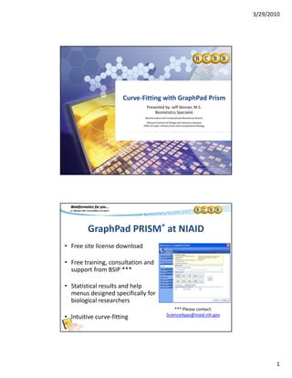
2. 3/29/2010
2
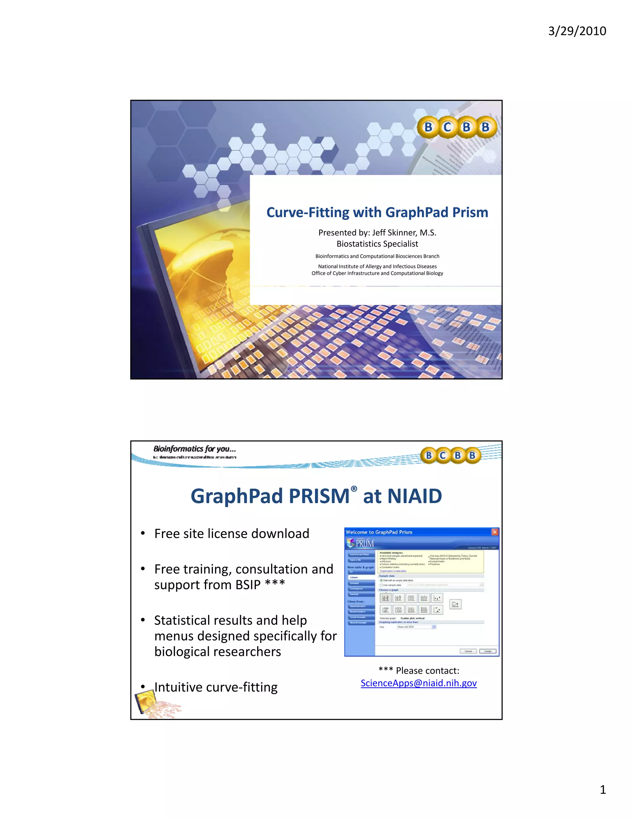
NIAID Site License
http://graphpad.com/paasl/index.cfm?sitecode=NIHNIAID
http://bioinformatics.niaid.nih.gov/
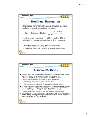
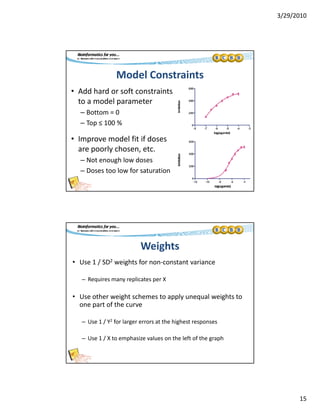
Nonlinear Regression
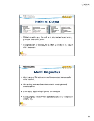
• Statistical technique commonly used for log dose s response
q y
curve‐fitting by biologists at NIAID
– Dose‐response studies
– Protein binding experiments
• Nonlinear regression is rarely studied in
statistics coursework
Sometimes mentioned briefl in a regression
log-dose vs response
-10 -8 -6 -4 -2
-100
0
100
200
300
400
500
No inhibitor
Inhibitor
log[Dose]
Response
dose vs. response
– Sometimes mentioned briefly in a regression
or linear models course
• Nonlinear regression is sometimes
omitted from statistical software or
poorly executed in software packages
0.0000 0.0001 0.0002 0.0003 0.0004
0
100
200
300
400
500
No inhibitor
Inhibitor
Dose
Response

3. 3/29/2010
3
Linear Versus Nonlinear
• There is an important distinction between a linear
relationship and a linear statistical model
– Linear or curved relationships describe how two variables
might be visualized together on a graph
– Linear models take the form Y = mX + b or Y = X + 
C d l ti hi b fit ith ith li• Curved relationships can be fit with either linear or
nonlinear statistical models
– Polynomial regression is linear in its parameters
– Sigmoidal dose‐response models are not linear
Simple Linear Regression
weight = -433.7 + 9.03  height + error
• Linear relationship between a
predictor, height, and a
response variable, weight, is
modeled by a straight line
– Model: Y = 0 + 1X + 
– Definition of a line: Y = mx + b
g g
Definition of a line: Y = mx + b
• The model is linear, so we can
estimate slope and y‐int using
calculus, or ordinary least
squares (OLS)

4. 3/29/2010
4
Polynomial Regression
binding = 0 + 1  (ligand) + 2  (ligand2) + … + 
• Fits a curved relationship using a
linear model
• Degree of polynomial indicates
the number of curves
– Quadratic (1 curve)
– Cubic (2 curves)
• High degree polynomials are best
fit by ANOVA models
Log‐transformations
growth = 0  exp{-1  age}   or ln(growth) = ln(0) - 1  age + ln()
• Imagine growth modeled by an
exponential equation with
multiplicative error
– I.e. errors get smaller as growth
decreases with increasing age
• Log transformation is often used
to “correct” a curved exponential
relationship

5. 3/29/2010
5
Nonlinear Regression
• Describes a nonlinear relationship between predictor
d i li tiand response using nonlinear equations
– E.g.
• Least squares equations do not have a closed form
solution (i.e. cannot use calculus to find estimates)
Response  Bottom
Top  Bottom
110 log EC50logX Hillslope
( )
• Estimates are found using iterative methods
– Pick initial values and converge to solution step‐by‐step
Iterative Methods
• Linear descent method starts with an initial value, then
“steps” away to minimize sums of squares (SS)steps away to minimize sums of squares (SS)
– If first positive step increases SS, step backwards
– If nth step increases SS, take smaller steps
– Linear descent is best for first steps from initial value
• Gauss‐Newton uses matrix algebra to minimize SS, as if it
were a change in “slope” from the initial value
– Gauss‐Newton is best for the last steps of minimization
• Levenberg‐Marquardt method starts with linear descent
and switches to Gauss‐Newton

6. 3/29/2010
6
Iterative Methods (continued)
• Strength of the iterative methods
– Can be used to fit any model
• Weaknesses of the iterative method
– Computationally slower than calculus method
– May find the local min, instead of global min
– May get “stuck” if model choice is poor
Local vs. Global Minima
L l
msofSquares
Global
Minimum
Local
Minimum
Finding a local
minimum implies
you have not
found the best
possible fit
Hillslope
Sum
possible fit

7. 3/29/2010
7
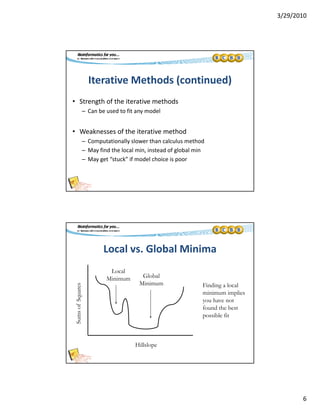
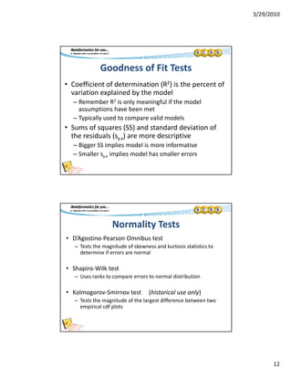
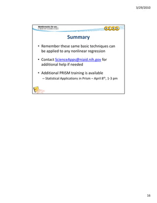
Dose‐Response Models
• Most commonly used model
among NIAID researchers
log-dose vs response
500
• Up to five parameters
– TOP and BOTTOM
– Log(EC50)
– Hillslope (default = 1)
– Symmetry (default = 1)
-10 -8 -6 -4 -2
-100
0
100
200
300
400
500
No inhibitor
Inhibitor
log[Agonist], M
• Concepts presented for dose‐
response models will apply to all
other nonlinear models Response  Bottom
Top  Bottom
110 logEC50logX Hillslope
Getting Started in PRISM
• Open a XY data table and
enter data
• Transform and normalize
data if necessary
• Open the nonlinear fit
menu in PRISM

8. 3/29/2010
8
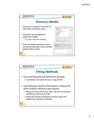
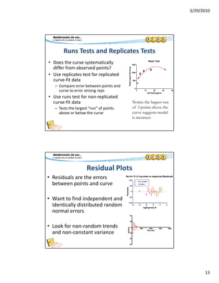
Why Use log(X) For Sigmoid Dose Response?
• Raw X values produce a
dose vs. response
500
Raw X values produce a
hyperbolic curve
– Large errors at the ascent
– Small errors at the plateau
• Log(X) values produce a log dose vs response
0.0000 0.0001 0.0002 0.0003 0.0004
0
100
200
300
400
No inhibitor
Inhibitor
Dose
Response
sigmoid “esse” curve
– Moderate errors throughout
– Best estimates of EC50
log-dose vs response
-10 -8 -6 -4 -2
-100
0
100
200
300
400
500
No inhibitor
Inhibitor
log[Dose]
Response
Importance of Log Transform

9. 3/29/2010
9
Choose a Model
• Choose an equation from the Fit
tab of the nonlinear mentab of the nonlinear menu
• Equations are grouped by
experiment types
– E.g. dose‐response, binding, …
• Click the details button to view
the actual equation and a sample
graph of the model
Fitting Methods
• Use Least Squares (LS) whenever possible
– LS produces the correct tests using all data
• Use Automatic Outlier Elimination or Robust Fit
when outliers influence your results
– Robust Fit uses all of your data, but cannot produce y , p
confidence intervals or tests
– Automatic Outlier Detection removes data and
applies least squares methods

10. 3/29/2010
10
Compare Groups or Models?
• Compare the fit of two different equations on
the same data set(s)
– Compare dose‐response models with and without a
variable slope parameter
– Compare different sets of constraints, etc.
• Compare best fit parameters between two or• Compare best fit parameters between two or
more groups in your experiment
– E.g. Compare EC50 between 2 or more groups
F‐test or AIC?
• Use extra sums of squares F‐test whenever the
i dtwo equations are nested:
– Dose‐response vs Dose‐Response (variable slope) is
nested, because one equation is a simplification of
the other equation
– Dose‐response versus binding equations is not
nested because the equations are unrelatednested, because the equations are unrelated
– Comparing 2 or more groups is always nested
• Use AIC if you are unsure about nesting

11. 3/29/2010
11
Statistical Output
• PRISM provides you the null and alternative hypotheses,
p‐values and conclusions
• Interpretation of the results is often spelled out for you in
plain language
Model Diagnostics
• Goodness‐of‐fit tests are used to compare two equally
lid d lvalid models
• Normality tests evaluate the model assumption of
normal errors
• Runs tests determine if errors are random
• Residual plots identify non‐constant variance, correlated
errors, etc.

12. 3/29/2010
12
Goodness of Fit Tests
• Coefficient of determination (R2) is the percent of
variation explained by the model
– Remember R2 is only meaningful if the model
assumptions have been met
– Typically used to compare valid models
• Sums of squares (SS) and standard deviation of
the residuals (sy.x) are more descriptive
– Bigger SS implies model is more informative
– Smaller sy.x implies model has smaller errors
Normality Tests
• D’Agostino‐Pearson Omnibus test
Tests the magnitude of skewness and kurtosis statistics to– Tests the magnitude of skewness and kurtosis statistics to
determine if errors are normal
• Shapiro‐Wilk test
– Uses ranks to compare errors to normal distribution
• Kolmogorov‐Smirnov test (historical use only)
– Tests the magnitude of the largest difference between two
empirical cdf plots

13. 3/29/2010
13
Runs Tests and Replicates Tests
• Does the curve systematically
diff f b d i t ?differ from observed points?
• Use replicates test for replicated
curve‐fit data
– Compare error between points and
curve to error among reps
• Use runs test for non‐replicated p
curve‐fit data
– Tests the largest “run” of points
above or below the curve
Notice the largest run
of 3 points above the
curve suggests model
is incorrect
Residual Plots
• Residuals are the errors
between points and curvebetween points and curve
• Want to find independent and
identically distributed random
normal errors
• Look for non‐random trends
and non‐constant variance

14. 3/29/2010
14
Improving Model Fit
• Change the initial values to aid convergence
• Limit the range of X or Y to eliminate outliers
• Add constraints to force the model to meet certain
criteria that improve model fit
– E.g. Bottom = 0%, Top = 100%, …
• Use a weighting scheme to combat non‐constant
variance or emphasize parts of the curve
Initial Values and Range
• Change the initial values of the parameters, if the
model does not converge
– Try the “Don’t Fit Curve” option on the diagnostics tab to find
better initial values
• Select the range of X values used curve‐fit to eliminate
outliers or invalid data pointsoutliers or invalid data points
• Select the range of the fitted curve to complete the
graphs and figures, if necessary

15. 3/29/2010
15
Model Constraints
• Add hard or soft constraints
to a model parameter
– Bottom = 0
– Top ≤ 100 %
• Improve model fit if doses
are poorly chosen, etc.
– Not enough low doses
– Doses too low for saturation
Weights
• Use 1 / SD2 weights for non‐constant variance
– Requires many replicates per X
• Use other weight schemes to apply unequal weights to
one part of the curve
– Use 1 / Y2 for larger errors at the highest responses
– Use 1 / X to emphasize values on the left of the graph

16. 3/29/2010
16
Summary
• Remember these same basic techniques can q
be applied to any nonlinear regression
• Contact ScienceApps@niaid.nih.gov for
additional help if needed
• Additional PRISM training is available
– Statistical Applications in Prism – April 8th, 1‐3 pm