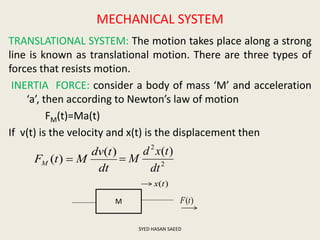
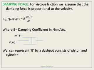
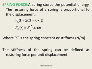
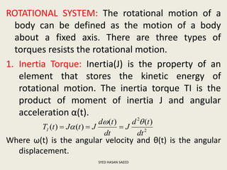
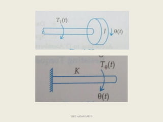
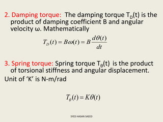
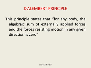
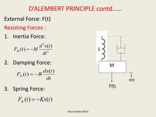
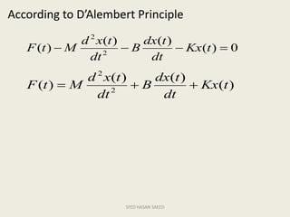
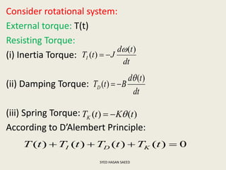
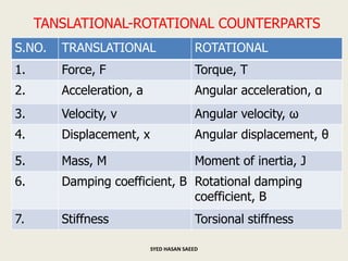
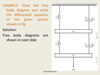
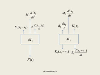
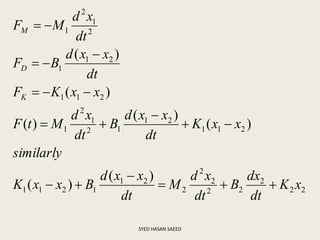
OUTLINE
 Definition of Transfer Function.
 Poles & Zeros.
 Characteristic Equation.
 Advantages of Transfer Function.
 Mechanical System (i) Translational System and
(ii) Rotational System.
 Free Body diagram.
 Transfer Function of Electrical, Mechanical
Systems.
 D’Alembert Principle.
SYED HASAN SAEED
TRANSFER FUNCTION
Definition: The transfer function is defined as the
ratio of Laplace transform of the output to the
Laplace transform of input with all initial
conditions are zero.
We can defined the transfer function as
SYED HASAN SAEED 2
)0.1(
.....
.....
)(
)(
)(
01
1
1
01
1
1



 



asasasa
bsbsbsb
sG
sR
sC
n
n
n
n
m
m
m
m
In equation (1.0), if the order of the denominator
polynomial is greater than the order of the numerator
polynomial then the transfer function is said to be
STRICTLY PROPER. If the order of both polynomials are
same, then the transfer function is PROPER. The transfer
function is said to be IMPROPER, if the order of
numerator polynomial is greater than the order of the
denominator polynomial.
CHARACTERISTIC EQUATION: The characteristic equation
can be obtained by equating the denominator
polynomial of the transfer function to zero. That is
SYED HASAN SAEED 3
0..... 01
1
1  
 asasasa n
n
n
n
POLES AND ZEROS OF A TRANSFER FUNCTION
POLES : The poles of G(s) are those values of ‘s’ which
make G(s) tend to infinity.
ZEROS: The zeros of G(s) are those values of ‘s’ which make
G(s) tend to zero.
If either poles or zeros coincide, then such type of poles or
zeros are called multiple poles or zeros, otherwise they
are known as simple poles or zeros.
For example, consider following transfer function
SYED HASAN SAEED 4
2
)4)(2(
)3(50
)(



sss
s
sG
This transfer function having the simple poles at s=0, s=-2,
multiple poles at s=-4 and simple zero at s=-3.
Advantages of Transfer Function:
1. Transfer function is a mathematical model of all system
components and hence of the overall system and
therefore it gives the gain of the system.
2. Since Laplace transform is used, it converts time domain
equations to simple algebraic equations.
3. With the help of transfer function, poles, zeros and
characteristic equation can be determine.
4. The differential equation of the system can be obtained
by replacing ‘s’ with d/dt.
SYED HASAN SAEED 5
DISADVANTAGES OF TRANSFER FUNCTION:
1. Transfer function cannot be defined for non-
linear system.
2. From the Transfer function , physical structure of
a system cannot determine.
3. Initial conditions loose their importance.
SYED HASAN SAEED 6
Find the transfer function of the given figure.
Solution:
Step 1: Apply KVL in mesh 1 and mesh 2
SYED HASAN SAEED 7
)2(
)1(


dt
di
Lv
dt
di
LRiv
o
i
Step 2: take Laplace transform of eq. (1) and (2)
Step 3: calculation of transfer function
Equation (5) is the required transfer function
SYED HASAN SAEED 8
)4()()(
)3()()()(


ssLIsV
ssLIsRIsV
o
i
)5(
)(
)(
)()(
)(
)(
)(





sLR
sL
sV
sV
sIsLR
ssLI
sV
sV
i
o
i
o
A system having input x(t) and output y(t) is represented by
Equation (1). Find the transfer function of the system.
Solution: taking Laplace transform of equation (1)
G(s) is the required transfer function
SYED HASAN SAEED
)1()(5
)(
)(4
)(
 tx
dt
tdx
ty
dt
tdy
4
5
)(
)(
)(
4
5
)(
)(
)5)(()4)((
)(5)()(4)(








s
s
sX
sY
sG
s
s
sX
sY
ssXssY
sXssXsYssY
The transfer function of the given system is given by
Find the differential equation of the system having input x(t) and
output y(t).
Solution:
Taking inverse Laplace transform, we have
Required differential equation is
SYED HASAN SAEED
32
14
)( 2



ss
s
sG
   
)(3)(2)()(4
32)(14)(
32
14
)(
)(
)(
2
2
2
sYssYssXssX
sssYssX
ss
s
sX
sY
sG





)(3
)(
2)(
)(
4 2
2
ty
dt
tdy
dt
dy
tx
dt
tdx

)(
)(
4)(3
)(
2
)(
2
2
tx
dt
tdx
ty
dt
tdy
dt
tyd

MECHANICAL SYSTEM
TRANSLATIONAL SYSTEM: The motion takes place along a strong
line is known as translational motion. There are three types of
forces that resists motion.
INERTIA FORCE: consider a body of mass ‘M’ and acceleration
‘a’, then according to Newton’s law of motion
FM(t)=Ma(t)
If v(t) is the velocity and x(t) is the displacement then
dt
tdv
MtFM
)(
)(  2
2
)(
dt
txd
M
SYED HASAN SAEED
M
)(tx
)(tF
DAMPING FORCE: For viscous friction we assume that the
damping force is proportional to the velocity.
FD(t)=B v(t)
Where B= Damping Coefficient in N/m/sec.
We can represent ‘B’ by a dashpot consists of piston and
cylinder.
SYED HASAN SAEED
dt
tdx
B
)(

)(tFD
)(tx
SPRING FORCE:A spring stores the potential energy.
The restoring force of a spring is proportional to
the displacement.
FK(t)=αx(t)=K x(t)
Where ‘K’ is the spring constant or stiffness (N/m)
The stiffness of the spring can be defined as
restoring force per unit displacement
SYED HASAN SAEED
 dttvKtFK )()(
ROTATIONAL SYSTEM: The rotational motion of a
body can be defined as the motion of a body
about a fixed axis. There are three types of
torques resists the rotational motion.
1. Inertia Torque: Inertia(J) is the property of an
element that stores the kinetic energy of
rotational motion. The inertia torque TI is the
product of moment of inertia J and angular
acceleration α(t).
Where ω(t) is the angular velocity and θ(t) is the angular
displacement.
SYED HASAN SAEED
2
2
)()(
)()(
dt
td
J
dt
td
JtJtTI

 
SYED HASAN SAEED
2. Damping torque: The damping torque TD(t) is the
product of damping coefficient B and angular
velocity ω. Mathematically
3. Spring torque: Spring torque Tθ(t) is the product
of torsional stiffness and angular displacement.
Unit of ‘K’ is N-m/rad
SYED HASAN SAEED
dt
td
BtBtTD
)(
)()(

 
)()( tKtT  
D’ALEMBERT PRINCIPLE
This principle states that “for any body, the
algebraic sum of externally applied forces
and the forces resisting motion in any given
direction is zero”
SYED HASAN SAEED
D’ALEMBERT PRINCIPLE contd……
External Force: F(t)
Resisting Forces :
1. Inertia Force:
2. Damping Force:
3. Spring Force:
SYED HASAN SAEED
2
2
)(
)(
dt
txd
MtFM 
dt
tdx
BtFD
)(
)( 
)()( tKxtFK 
M
F(t)
X(t)
According to D’Alembert Principle
SYED HASAN SAEED
0)(
)()(
)( 2
2
 tKx
dt
tdx
B
dt
txd
MtF
)(
)()(
)( 2
2
tKx
dt
tdx
B
dt
txd
MtF 
Consider rotational system:
External torque: T(t)
Resisting Torque:
(i) Inertia Torque:
(ii) Damping Torque:
(iii) Spring Torque:
According to D’Alembert Principle:
SYED HASAN SAEED
dt
td
JtTI
)(
)(


dt
td
BtTD
)(
)(


)()( tKtTK 
0)()()()(  tTtTtTtT KDI
SYED HASAN SAEED
0)(
)()(
)(  tK
dt
td
B
dt
td
JtT 

)(
)()(
)( tK
dt
td
B
dt
td
JtT 


D'Alembert Principle for rotational motion states
that
“For anybody, the algebraic sum of externally
applied torques and the torque resisting rotation
about any axis is zero.”
TANSLATIONAL-ROTATIONAL COUNTERPARTS
S.NO. TRANSLATIONAL ROTATIONAL
1. Force, F Torque, T
2. Acceleration, a Angular acceleration, α
3. Velocity, v Angular velocity, ω
4. Displacement, x Angular displacement, θ
5. Mass, M Moment of inertia, J
6. Damping coefficient, B Rotational damping
coefficient, B
7. Stiffness Torsional stiffness
SYED HASAN SAEED
EXAMPLE: Draw the free
body diagram and write
the differential equation
of the given system
shown in fig.
Solution:
Free body diagrams are
shown in next slide
SYED HASAN SAEED
SYED HASAN SAEED
2
1
2
1
dt
xd
M
)( 211 xxK 
dt
xxd
B
)( 21
1

)(tF
1M 2M
)( 211 xxK 
dt
xxd
B
)( 21
1

2
2
2
2
dt
xd
M
dt
dx
B 2
2 22 xK
22
2
22
2
2
2
21
1211
211
21
12
1
2
1
211
21
1
2
1
2
1
)(
)(
)(
)(
)(
)(
)(
xK
dt
dx
B
dt
xd
M
dt
xxd
BxxK
similarly
xxK
dt
xxd
B
dt
xd
MtF
xxKF
dt
xxd
BF
dt
xd
MF
K
D
M










SYED HASAN SAEED
Figure
Write the differential equations describing the
dynamics of the systems shown in figure and
find the ratio
SYED HASAN SAEED
)(
)(2
sF
sX
FREE BODY DAIGRAMS
SYED HASAN SAEED
1M
2
1
2
1
dt
xd
M
)( 211 xxK 
)(tF
2M
2
2
2
dt
xd
M
22 xK
)( 211 xxK 
Differential equations are
SYED HASAN SAEED
2
2
2
222211
2112
1
2
1
)(
)()(
dt
xd
MxKxxK
xxK
dt
xd
MtF


LaplaceTransform of above equations
)()()()(
)()()()(
2
2
2222111
21111
2
1
sXsMsXKsXKsXK
sXKsXKsXsMsF


Solve equationsabove for
2
11
2
1212
2
12
))(()(
)(
KMsKKKMs
K
sF
sX


)(
)(2
sF
sX
THANK YOU
SYED HASAN SAEED

Transfer fn mech. systm

  • 1.
    OUTLINE  Definition ofTransfer Function.  Poles & Zeros.  Characteristic Equation.  Advantages of Transfer Function.  Mechanical System (i) Translational System and (ii) Rotational System.  Free Body diagram.  Transfer Function of Electrical, Mechanical Systems.  D’Alembert Principle. SYED HASAN SAEED
  • 2.
    TRANSFER FUNCTION Definition: Thetransfer function is defined as the ratio of Laplace transform of the output to the Laplace transform of input with all initial conditions are zero. We can defined the transfer function as SYED HASAN SAEED 2 )0.1( ..... ..... )( )( )( 01 1 1 01 1 1         asasasa bsbsbsb sG sR sC n n n n m m m m
  • 3.
    In equation (1.0),if the order of the denominator polynomial is greater than the order of the numerator polynomial then the transfer function is said to be STRICTLY PROPER. If the order of both polynomials are same, then the transfer function is PROPER. The transfer function is said to be IMPROPER, if the order of numerator polynomial is greater than the order of the denominator polynomial. CHARACTERISTIC EQUATION: The characteristic equation can be obtained by equating the denominator polynomial of the transfer function to zero. That is SYED HASAN SAEED 3 0..... 01 1 1    asasasa n n n n
  • 4.
    POLES AND ZEROSOF A TRANSFER FUNCTION POLES : The poles of G(s) are those values of ‘s’ which make G(s) tend to infinity. ZEROS: The zeros of G(s) are those values of ‘s’ which make G(s) tend to zero. If either poles or zeros coincide, then such type of poles or zeros are called multiple poles or zeros, otherwise they are known as simple poles or zeros. For example, consider following transfer function SYED HASAN SAEED 4 2 )4)(2( )3(50 )(    sss s sG
  • 5.
    This transfer functionhaving the simple poles at s=0, s=-2, multiple poles at s=-4 and simple zero at s=-3. Advantages of Transfer Function: 1. Transfer function is a mathematical model of all system components and hence of the overall system and therefore it gives the gain of the system. 2. Since Laplace transform is used, it converts time domain equations to simple algebraic equations. 3. With the help of transfer function, poles, zeros and characteristic equation can be determine. 4. The differential equation of the system can be obtained by replacing ‘s’ with d/dt. SYED HASAN SAEED 5
  • 6.
    DISADVANTAGES OF TRANSFERFUNCTION: 1. Transfer function cannot be defined for non- linear system. 2. From the Transfer function , physical structure of a system cannot determine. 3. Initial conditions loose their importance. SYED HASAN SAEED 6
  • 7.
    Find the transferfunction of the given figure. Solution: Step 1: Apply KVL in mesh 1 and mesh 2 SYED HASAN SAEED 7 )2( )1(   dt di Lv dt di LRiv o i
  • 8.
    Step 2: takeLaplace transform of eq. (1) and (2) Step 3: calculation of transfer function Equation (5) is the required transfer function SYED HASAN SAEED 8 )4()()( )3()()()(   ssLIsV ssLIsRIsV o i )5( )( )( )()( )( )( )(      sLR sL sV sV sIsLR ssLI sV sV i o i o
  • 9.
    A system havinginput x(t) and output y(t) is represented by Equation (1). Find the transfer function of the system. Solution: taking Laplace transform of equation (1) G(s) is the required transfer function SYED HASAN SAEED )1()(5 )( )(4 )(  tx dt tdx ty dt tdy 4 5 )( )( )( 4 5 )( )( )5)(()4)(( )(5)()(4)(         s s sX sY sG s s sX sY ssXssY sXssXsYssY
  • 10.
    The transfer functionof the given system is given by Find the differential equation of the system having input x(t) and output y(t). Solution: Taking inverse Laplace transform, we have Required differential equation is SYED HASAN SAEED 32 14 )( 2    ss s sG     )(3)(2)()(4 32)(14)( 32 14 )( )( )( 2 2 2 sYssYssXssX sssYssX ss s sX sY sG      )(3 )( 2)( )( 4 2 2 ty dt tdy dt dy tx dt tdx  )( )( 4)(3 )( 2 )( 2 2 tx dt tdx ty dt tdy dt tyd 
  • 11.
    MECHANICAL SYSTEM TRANSLATIONAL SYSTEM:The motion takes place along a strong line is known as translational motion. There are three types of forces that resists motion. INERTIA FORCE: consider a body of mass ‘M’ and acceleration ‘a’, then according to Newton’s law of motion FM(t)=Ma(t) If v(t) is the velocity and x(t) is the displacement then dt tdv MtFM )( )(  2 2 )( dt txd M SYED HASAN SAEED M )(tx )(tF
  • 12.
    DAMPING FORCE: Forviscous friction we assume that the damping force is proportional to the velocity. FD(t)=B v(t) Where B= Damping Coefficient in N/m/sec. We can represent ‘B’ by a dashpot consists of piston and cylinder. SYED HASAN SAEED dt tdx B )(  )(tFD )(tx
  • 13.
    SPRING FORCE:A springstores the potential energy. The restoring force of a spring is proportional to the displacement. FK(t)=αx(t)=K x(t) Where ‘K’ is the spring constant or stiffness (N/m) The stiffness of the spring can be defined as restoring force per unit displacement SYED HASAN SAEED  dttvKtFK )()(
  • 14.
    ROTATIONAL SYSTEM: Therotational motion of a body can be defined as the motion of a body about a fixed axis. There are three types of torques resists the rotational motion. 1. Inertia Torque: Inertia(J) is the property of an element that stores the kinetic energy of rotational motion. The inertia torque TI is the product of moment of inertia J and angular acceleration α(t). Where ω(t) is the angular velocity and θ(t) is the angular displacement. SYED HASAN SAEED 2 2 )()( )()( dt td J dt td JtJtTI   
  • 15.
  • 16.
    2. Damping torque:The damping torque TD(t) is the product of damping coefficient B and angular velocity ω. Mathematically 3. Spring torque: Spring torque Tθ(t) is the product of torsional stiffness and angular displacement. Unit of ‘K’ is N-m/rad SYED HASAN SAEED dt td BtBtTD )( )()(    )()( tKtT  
  • 17.
    D’ALEMBERT PRINCIPLE This principlestates that “for any body, the algebraic sum of externally applied forces and the forces resisting motion in any given direction is zero” SYED HASAN SAEED
  • 18.
    D’ALEMBERT PRINCIPLE contd…… ExternalForce: F(t) Resisting Forces : 1. Inertia Force: 2. Damping Force: 3. Spring Force: SYED HASAN SAEED 2 2 )( )( dt txd MtFM  dt tdx BtFD )( )(  )()( tKxtFK  M F(t) X(t)
  • 19.
    According to D’AlembertPrinciple SYED HASAN SAEED 0)( )()( )( 2 2  tKx dt tdx B dt txd MtF )( )()( )( 2 2 tKx dt tdx B dt txd MtF 
  • 20.
    Consider rotational system: Externaltorque: T(t) Resisting Torque: (i) Inertia Torque: (ii) Damping Torque: (iii) Spring Torque: According to D’Alembert Principle: SYED HASAN SAEED dt td JtTI )( )(   dt td BtTD )( )(   )()( tKtTK  0)()()()(  tTtTtTtT KDI
  • 21.
    SYED HASAN SAEED 0)( )()( )( tK dt td B dt td JtT   )( )()( )( tK dt td B dt td JtT    D'Alembert Principle for rotational motion states that “For anybody, the algebraic sum of externally applied torques and the torque resisting rotation about any axis is zero.”
  • 22.
    TANSLATIONAL-ROTATIONAL COUNTERPARTS S.NO. TRANSLATIONALROTATIONAL 1. Force, F Torque, T 2. Acceleration, a Angular acceleration, α 3. Velocity, v Angular velocity, ω 4. Displacement, x Angular displacement, θ 5. Mass, M Moment of inertia, J 6. Damping coefficient, B Rotational damping coefficient, B 7. Stiffness Torsional stiffness SYED HASAN SAEED
  • 23.
    EXAMPLE: Draw thefree body diagram and write the differential equation of the given system shown in fig. Solution: Free body diagrams are shown in next slide SYED HASAN SAEED
  • 24.
    SYED HASAN SAEED 2 1 2 1 dt xd M )(211 xxK  dt xxd B )( 21 1  )(tF 1M 2M )( 211 xxK  dt xxd B )( 21 1  2 2 2 2 dt xd M dt dx B 2 2 22 xK
  • 25.
  • 26.
    Figure Write the differentialequations describing the dynamics of the systems shown in figure and find the ratio SYED HASAN SAEED )( )(2 sF sX
  • 27.
    FREE BODY DAIGRAMS SYEDHASAN SAEED 1M 2 1 2 1 dt xd M )( 211 xxK  )(tF 2M 2 2 2 dt xd M 22 xK )( 211 xxK 
  • 28.
    Differential equations are SYEDHASAN SAEED 2 2 2 222211 2112 1 2 1 )( )()( dt xd MxKxxK xxK dt xd MtF   LaplaceTransform of above equations )()()()( )()()()( 2 2 2222111 21111 2 1 sXsMsXKsXKsXK sXKsXKsXsMsF   Solve equationsabove for 2 11 2 1212 2 12 ))(()( )( KMsKKKMs K sF sX   )( )(2 sF sX
  • 29.