LECTURE (2)
Mathematical Modeling of
Systems
Assist. Prof. Amr E. Mohamed
Objectives
 In this lecture, we lead you through a study of mathematical models of
physical systems.
 After completing the chapter, you should be able to
 Describe a physical system in terms of differential equations.
 Understand the way these equations are obtained.
 Realize the use of physical laws governing a particular system such as
 Newton’s law for mechanical systems and Kirchhoff’s laws for electrical
systems.
 Realize that deriving mathematical models is the most important part of
the entire analysis of control systems.
2
Mathematical Model
 Mathematical modeling of any control system is the first and foremost task that a
control engineer has to accomplish for design and analysis of any control engineering
problem.
 A mathematical model of a dynamic system is defined as a set of differential equations
that represents the dynamics of the system accurately, or at least fairly well.
 Note that a mathematical model is not unique to a given system. A system may be
represented in many different ways and, therefore, may have many mathematical
models, depending on one’s perspective. For example,
 In optimal control problems, it is good to use state-space representations.
 On the other hand, for the transient-response or frequency-response analysis of single-
input-single-output, linear, time-invariant systems, the transfer function
representation may be more convenient than any other.
 Once a mathematical model of a system is obtained, various analytical and
computational techniques may be used for analysis and synthesis purposes. Because
the systems under consideration are dynamic in nature, the equations are usually
differential equations. If these equations can be linearized, then the Laplace
transform may be utilized to simplify the method of solution. 3
Different Mathematical Models
 Commonly used mathematical models are
 Differential equation model (Time Domain).
 Transfer function model (S-Domain).
 State space model (Time Domain).
 Use of the models depends on the application. For example, to find the
transient or steady state response of SISO (Single Input Single Output)
LTI (Linear Time Invariant) system transfer function model is useful. On
the other hand for optimal control application state space model is
useful.
4
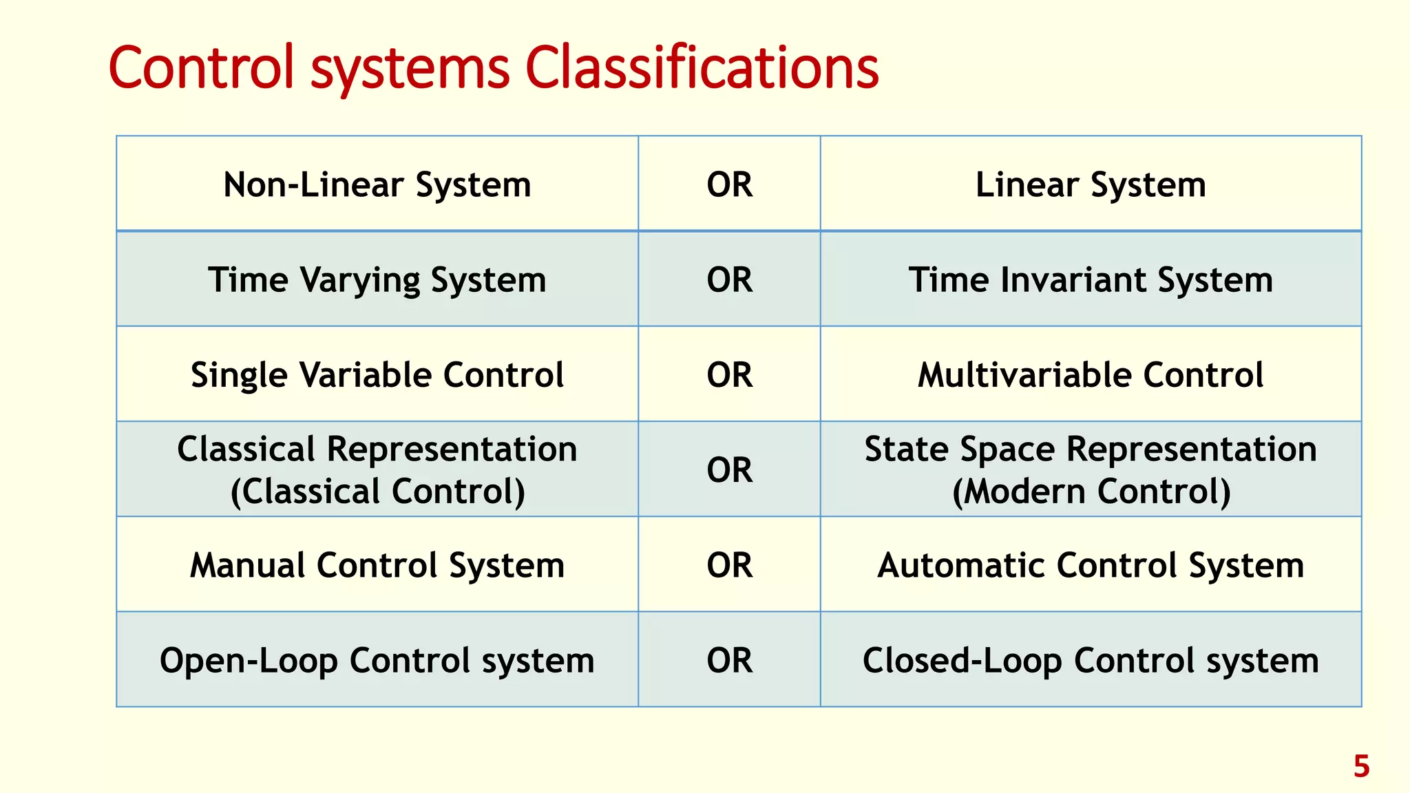
Control systems Classifications
5
Non-Linear System OR Linear System
Time Varying System OR Time Invariant System
Single Variable Control OR Multivariable Control
Classical Representation
(Classical Control)
OR
State Space Representation
(Modern Control)
Manual Control System OR Automatic Control System
Open-Loop Control system OR Closed-Loop Control system
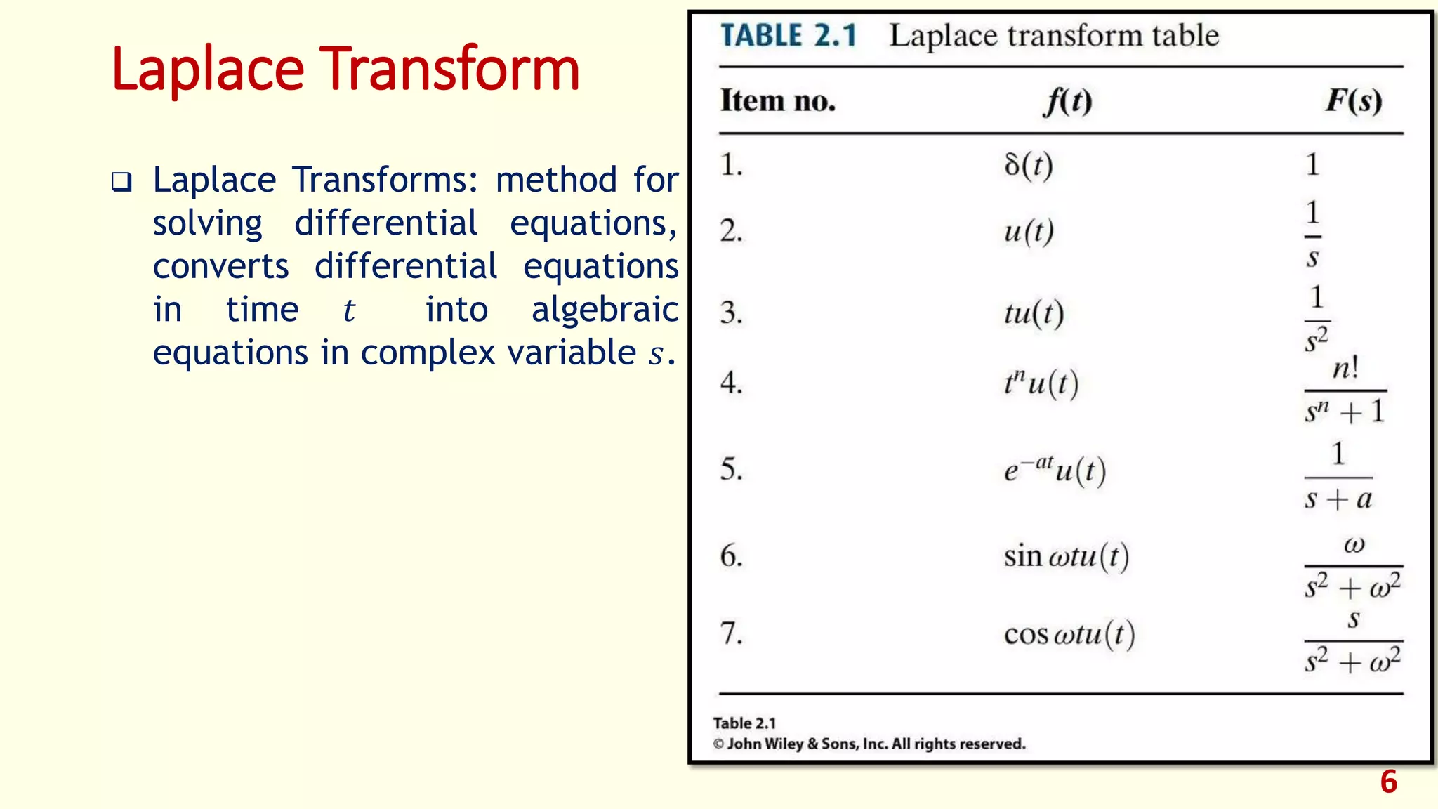
Laplace Transform
 Laplace Transforms: method for
solving differential equations,
converts differential equations
in time 𝑡 into algebraic
equations in complex variable 𝑠.
6
Laplace
Transform
Properties
7
The approach to dynamic system problems can be as follows:
1. Define the system and its components.
2. Formulate the mathematical model and list the necessary assumptions
3. Write the differential equations describing the model.
4. Solve the equations for the desired output variables.
5. Examine the solution and the assumptions.
6. If necessary reanalyze or redesign the system.
8
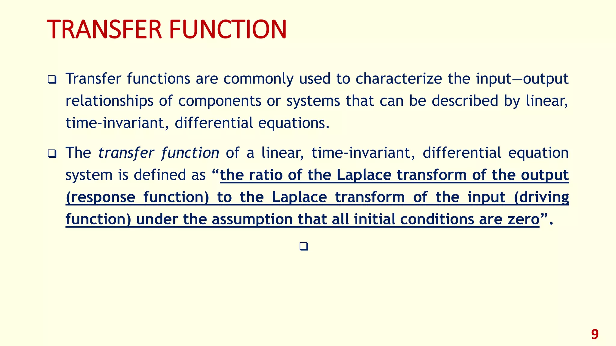
TRANSFER FUNCTION
 Transfer functions are commonly used to characterize the input—output
relationships of components or systems that can be described by linear,
time-invariant, differential equations.
 The transfer function of a linear, time-invariant, differential equation
system is defined as “the ratio of the Laplace transform of the output
(response function) to the Laplace transform of the input (driving
function) under the assumption that all initial conditions are zero”.

9
TRANSFER FUNCTION
 The general form of the differential equation for LTI-System is given by
𝒂 𝟎 𝒚
(𝒏)
+ 𝒂 𝟏 𝒚
(𝒏−𝟏)
+ … + 𝒂 𝒏−𝟏 𝒚 + 𝒂 𝒏 𝒚 = 𝒃 𝟎 𝒙
(𝒎)
+ 𝒃 𝟏 𝒙
(𝒎−𝟏)
+ … + 𝒃 𝒎−𝟏 𝒙 + 𝒃 𝒎 𝒙
 where y is the system output and x is the input of the System
 The transfer function of this system is obtained by taking the Laplace
transforms of both sides of Equation (under the assumption that all initial
conditions are zero),
𝑎0 𝑆 𝑛
𝑌 𝑠 + ⋯ + 𝑎 𝑛−1 𝑆1
𝑌 𝑠 + 𝑎 𝑛 𝑌 𝑠 = 𝑏0 𝑆 𝒎
𝑿(𝑠) + ⋯ + 𝑏 𝑚−1 𝑆 𝟏
𝑿(𝑠) + 𝑏 𝑚 𝑿(𝒔)
Then: 𝑎0 𝑆 𝑛
+ ⋯ + 𝑎 𝑛−1 𝑆1
+ 𝑎 𝑛 𝑌 𝑠 = 𝑏0 𝑆 𝒎
+ ⋯ + 𝑏 𝑚−1 𝑆 𝟏
+ 𝑏 𝑚 𝑿(𝒔)
10
TRANSFER FUNCTION
 Then the transfer function is
𝑻𝒓𝒂𝒏𝒔𝒇𝒆𝒓 𝑭𝒖𝒏𝒄𝒕𝒊𝒐𝒏 = 𝑮 𝒔 =
𝑳𝒂𝒑𝒍𝒂𝒄𝒆 𝒐𝒇 𝑶𝒖𝒕𝒑𝒖𝒕
𝑳𝒂𝒑𝒍𝒂𝒄𝒆 𝒐𝒇 𝑰𝒏𝒑𝒖𝒕 𝑨𝒔𝒔𝒖𝒎𝒊𝒏𝒈 𝒁𝒆𝒓𝒐 𝒊𝒏𝒊𝒕𝒊𝒂𝒍 𝑪𝒐𝒏𝒅𝒊𝒕𝒊𝒐𝒏
𝐺 𝑠 =
𝑌(𝑠)
𝑋(𝑠)
=
𝑏0 𝑆 𝒎 + ⋯ + 𝑏 𝑚−1 𝑆 𝟏 + 𝑏 𝑚
𝑎0 𝑆 𝑛 + 𝑎1 𝑆 𝑛−1 + ⋯ + 𝑎 𝑛−1 𝑆1 + 𝑎 𝑛
 Poles: are roots of the denominator (Values of s such that transfer
function becomes infinite)
 Zeros: are roots of the numerator (Values of s such that transfer
function becomes 0)
11
To derive the transfer function
1. Write the differential equation for the system.
2. Take the Laplace transform of the differential equation, assuming all
initial conditions are zero.
3. Take the ratio of the output Y(s) to the input R(s). This ratio is the
transfer function.
12
Describing Differential Equations for Electrical and
Electronic Elements
13
Electrical Circuits
14
Op Amps in system control
 Signal amplification in the sensor circuits
 Filters used for compensation purposes
 Modeling of the “real world” systems
 Lead or lag networks
 Design of controllers
15
u(s)
e(t) OPAMP+
-
OUT
R1
R2
u(t)
e(t)
OPAMP
+
-
OUT
R2
R1
Inverting amplifier Non-inverting amplifier
   te
R
R
tu
1
2
    te
R
R
tu 






1
2
1
Op Amps in system control
16
Summation circuit
        tetete
R
R
tu 321
1
2
OPAMP+
-
OUT
R1
R1
R1
R2
u(t)
e1(t)
e2(t)
e3(t)
U(s)
E(s) OPAMP+
-
OUT
Z1
Z2
 
  1
2
Z
Z
sE
sU

Transfer function of op amp
Op Amps in system control
17
U(s)
E(s)
C1
OPAMP+
-
OUT
R1
Integrator
 
  ITssCRZ
Z
sE
sU


11
111
2
Differentiator
 
  11
2
1
2


sCR
sCR
Z
Z
sE
sU
Op Amp lead-or-lag network
18
111
1
1


sCR
R
Z 122
2
2


sCR
R
Z
U(s)
E(s)
C2
OPAMP+
-
OUT
R1
R2
C1
 
  1
11
22
2
1
2 1
1 R
sCR
sCR
R
Z
Z
sE
sU 


Op Amp lead-lag network
19
 
  1
1
131
311
1



sCRR
RsCR
Z
 
  1
1
242
422
2



sCRR
RsCR
Z
Eo(s)
Ei(s)
C2
OPAMP+
-
OUT
R3
R4
C1
R1
R2
OPAMP+
-
OUT
R5
R6
Example: Write the integodifferential equations and the
transfer function of the following circuit
20
v(t))ii(
dt
d
LRi  2111
0
0
2
1
1222
 
t
dti
c
)ii(
dt
d
LRi
Take Laplace Transform of both
sides then find G(s) = I2(s)/V(s)
Describing Differential Equations for Translation
Mechanical Elements
21
Example: Write the differential equations and the transfer
function of the Spring Mass Damping System shown
22
s-domain
)()( sFsV
s
K
fMs v 






K
vf
M
)(tf
)(tv
)()(
)()(
2
2
tftKx
dt
tdx
f
dt
txd
M v 
differential equation
transfer function
 KsfMs
s
sF
sV
v 
 2
)(
)(
Example: Write the differential equations to model the
system shown
23
1K
1M
)(tf )(1 tx
2K
vf 2M
)(2 tx
3K
For the Mass M1
K2 (x1(t) – x2(t)) + K1x1(t) + fv d/dt (x1(t) – x2(t)) + M1 d2/dt2 x1(t) = f(t)
For the Mass M2
K2 (x1(t) – x2(t)) + fv d/dt (x1(t) – x2(t)) = K3x2(t) + M2 d2/dt2 x2(t)
Input
Output
Describing Differential Equations for Rotational
Mechanical Elements
24
Transfer Function for:
(a) Angular (b) Torque Displacement
Describing Differential Equations for Electro Mechanical
Elements
25
DC Motor
dt
td
Kv m
bb
)(
 Vb = Back electomotive force
Kb = the constant back emf
)()( sIKsT atm 
Tm = Torque of the motor
Kt = motor torque constant
)()()( 2
ssDsJsT mmmm 
Mechanical Relation
Electrical Relation








)(
1)(
)(
a
bt
m
m
mat
a
m
R
KK
D
J
ss
JRK
sE
s
Ia(s) = (Ea(s)-Vb(s))/(Ra+sLa)
The Transfer Function is
Block Diagram Models
 A block diagram of a system is a pictorial representation of the
functions performed by each component and of the flow of signals.
 Such diagram depicts the interrelationships that exist among the various
components. Differing from a purely abstract mathematical
representation, a block diagram has the advantage of indicating more
realistically the signal flows of the actual system.
 Transfer function can be represented as a block diagram:
26
)(sR )(sC
0
1
1
0
1
1
asasa
bsbsb
n
n
n
n
m
m
m
m








Components Of a block diagram for a LTI system
27
Procedures for drawing block diagram
1. Write the equations that describe the dynamic behavior for each
component.
2. Take Laplace transform of these equations, assuming zero initial
conditions.
3. Represent each Laplace-transformed equation individually in block
form.
4. Assembly the elements into a complete block diagram.
28
Example:
 Example derive the D.E. and the transfer function then draw the block
diagram for the following circuit:
 Take Laplace transform:
29
R
Cei eo
i
R
sEsE
R
tete
sI oioi )()()()(
)(







 
 L
C
idt
e
R
ee
i o
oi 


   
Cs
sI
C
idt
sEo 









L
Block Diagram Reduction
 Rules for reduction of the block diagram:
1. Any number of cascaded blocks can be reduced by a single block
representing transfer function being a product of transfer functions of
all cascaded blocks.
30
Block Diagram Reduction
2. Moving a summing point
31
(a) Behind the block
(b) Ahead of the block
Block Diagram Reduction
3. Moving a pickoff point
32
(a) Behind the block
(b) Ahead of the block
Block Diagram Reduction
4. Equivalent transfer function for parallel subsystems is the sum of
their transfer functions
33
Block Diagram Reduction
5. Feedback control system
34
Example reduce the following block diagram:
35
R
_+
_
+1G 2G 3G
1H
2H
+
+
C
Moving the summing point ahead of G1, we have:
36
R
_+
_
+ 1G 2G 3G
1H
1
2
G
H
+
+
C
Combing G1 and G2 in Cascade, we get:
37
R
_+
_
+ 21GG 3G
1H
1
2
G
H
+
+
C
Eliminating the feedback loop G1, G2 and H1 we get:
38
R
_+
_
+ 21GG 3G
1H
1
2
G
H
+
+
C
Combing the two blocks in Cascade, we get
39
R
_+
_
+
121
21
1 HGG
GG
 3G
1
2
G
H
C
Similarly eliminating the second feedback loop we get:
40
R
_+
_
+
121
321
1 HGG
GGG

1
2
G
H
C
Similarly eliminating the third feedback loop we get:
41
R
_+
232121
321
1 HGGHGG
GGG

C
The system is reduced to the following block diagram:
42
R
321232121
321
1 GGGHGGHGG
GGG

C
Conclusions of block diagram reduction Technique
1. Numerator of the closed-loop transfer function C(s)/R(s) is the product
of the transfer functions of the feedforward path.
2. The denominator of the closed-loop transfer function C(s)/R(s) is equal
to:
1 − Σ( 𝑝𝑟𝑜𝑑𝑢𝑐𝑡 𝑜𝑓 𝑡ℎ𝑒 𝑡𝑟𝑎𝑛𝑠𝑓𝑒𝑟 𝑓𝑢𝑛𝑐𝑡𝑖𝑜𝑛𝑠 𝑎𝑟𝑜𝑢𝑛𝑑 𝑒𝑎𝑐ℎ 𝑙𝑜𝑜𝑝)
3. The positive feedback loop yields a negative term in the denominator.
43
Example of system with two inputs R(s) and D(s)
1. Find 𝑌1(𝑠)/𝐷(𝑠) when 𝑅(𝑠) = 0
2. Find 𝑌2(𝑠)/𝑅(𝑠) when 𝐷(𝑠) = 0
3. Deduce the total response 𝑌(𝑠) of the
control system when R(s) and D(s) ≠ 0
𝑌1 𝑠
𝐷 𝑠 𝑅 𝑠 =0
=
𝐺2
1 + 𝐺2(𝐻1 − 𝐻2)
𝑌2 𝑠
𝑅 𝑠 𝐷 𝑠 =0
=
𝐺1 𝐺2
1 + 𝐺2(𝐻1 − 𝐻2)
𝑌 𝑠 = 𝑌1 𝑠 + 𝑌2 𝑠 =
𝑌1 𝑠
𝐷 𝑠 𝑅 𝑠 =0
. 𝐷(𝑠) +
𝑌2 𝑠
𝑅 𝑠 𝐷 𝑠 =0
. 𝑅(𝑠)
𝑌 𝑠 =
𝐺2
1 + 𝐺2 𝐻1 − 𝐻2
𝐷 𝑠 +
𝐺1 𝐺2
1 + 𝐺2 𝐻1 − 𝐻2
𝑅(𝑠)
44
Signal Flow Graph Models
 Definitions:
45
input node (source)
b1x a
2x
c
4x
d
1
3x
3x
output node (sink)
mixed node
input node (source)
mixed node
forward path
path
loop
branch
node
transmittance
Signal Flow Graph Models
 Node: a point representing a signal or variable.
 Branch: unidirectional line segment joining two nodes.
 Path: a branch or a continuous sequence of branches that can be
traversed from one node to another node.
 Loop: a closed path that originates and terminates on the same node
and along the path no node is met twice.
 Nontouching loops: two loops are said to be nontouching if they do not
have a common node.
46
Flow graphs of control systems
47
)(sR
)(sG
)(sC
)(sG)(sR )(sC
block diagram signal flow graph
)(sR
_+
)(sH
)(sG
)(sC)(sE
)(sG
)(sR
)(sC
1
)(sE )(sH
Mason’s Signal Flow Graph Gain Formula
 The transfer function T(s) of a closed loop control system is:
 Where
∆ = 1 – Σ(All different loop gains)
+ Σ(Gain products of all combinations of two non-touching loops)
- Σ(Gain products of all combinations of three non-touching loops)
+ …
 Pk : The paths connecting the input R(s) and the output Y(s)
 ∆k : is ∆ with the loops touching the kth path removed
48



k kpk
sR
sY
sT
)(
)(
)(
Example:
1. Calculate forward path transfer function Pk for each forward path k.
2. Calculate all loop TF’s.
3. Consider nontouching loops 2 at a time.
 Loops L1 do not touch Loops L3 and L4
 Loops L2 do not touch Loops L3 and L4
49
87652
43211
GGGGP
GGGGP


774663
332221
,
,,
HGLHGL
GHLHGL


Example:
5. Calculate Δ.
6. Calculate Δk for each forward path.
7. The TF of the system is
50
   4232413143211 LLLLLLLLLLLL 
 
 212
431
1
1
LL
LL


   
   423241314321
2187654343212211
1
11
)(
)(
)(
LLLLLLLLLLLL
LLGGGGLLGGGGPP
sT
sR
sY






Block Diagram to Signal Flow Graph
 The SFG can be constructed from the block diagram as show in the
following example:
 To get the transfer function, we use the Mason’s Gain Formula. 51
52

Modern Control - Lec 02 - Mathematical Modeling of Systems

  • 1.
    LECTURE (2) Mathematical Modelingof Systems Assist. Prof. Amr E. Mohamed
  • 2.
    Objectives  In thislecture, we lead you through a study of mathematical models of physical systems.  After completing the chapter, you should be able to  Describe a physical system in terms of differential equations.  Understand the way these equations are obtained.  Realize the use of physical laws governing a particular system such as  Newton’s law for mechanical systems and Kirchhoff’s laws for electrical systems.  Realize that deriving mathematical models is the most important part of the entire analysis of control systems. 2
  • 3.
    Mathematical Model  Mathematicalmodeling of any control system is the first and foremost task that a control engineer has to accomplish for design and analysis of any control engineering problem.  A mathematical model of a dynamic system is defined as a set of differential equations that represents the dynamics of the system accurately, or at least fairly well.  Note that a mathematical model is not unique to a given system. A system may be represented in many different ways and, therefore, may have many mathematical models, depending on one’s perspective. For example,  In optimal control problems, it is good to use state-space representations.  On the other hand, for the transient-response or frequency-response analysis of single- input-single-output, linear, time-invariant systems, the transfer function representation may be more convenient than any other.  Once a mathematical model of a system is obtained, various analytical and computational techniques may be used for analysis and synthesis purposes. Because the systems under consideration are dynamic in nature, the equations are usually differential equations. If these equations can be linearized, then the Laplace transform may be utilized to simplify the method of solution. 3
  • 4.
    Different Mathematical Models Commonly used mathematical models are  Differential equation model (Time Domain).  Transfer function model (S-Domain).  State space model (Time Domain).  Use of the models depends on the application. For example, to find the transient or steady state response of SISO (Single Input Single Output) LTI (Linear Time Invariant) system transfer function model is useful. On the other hand for optimal control application state space model is useful. 4
  • 5.
    Control systems Classifications 5 Non-LinearSystem OR Linear System Time Varying System OR Time Invariant System Single Variable Control OR Multivariable Control Classical Representation (Classical Control) OR State Space Representation (Modern Control) Manual Control System OR Automatic Control System Open-Loop Control system OR Closed-Loop Control system
  • 6.
    Laplace Transform  LaplaceTransforms: method for solving differential equations, converts differential equations in time 𝑡 into algebraic equations in complex variable 𝑠. 6
  • 7.
  • 8.
    The approach todynamic system problems can be as follows: 1. Define the system and its components. 2. Formulate the mathematical model and list the necessary assumptions 3. Write the differential equations describing the model. 4. Solve the equations for the desired output variables. 5. Examine the solution and the assumptions. 6. If necessary reanalyze or redesign the system. 8
  • 9.
    TRANSFER FUNCTION  Transferfunctions are commonly used to characterize the input—output relationships of components or systems that can be described by linear, time-invariant, differential equations.  The transfer function of a linear, time-invariant, differential equation system is defined as “the ratio of the Laplace transform of the output (response function) to the Laplace transform of the input (driving function) under the assumption that all initial conditions are zero”.  9
  • 10.
    TRANSFER FUNCTION  Thegeneral form of the differential equation for LTI-System is given by 𝒂 𝟎 𝒚 (𝒏) + 𝒂 𝟏 𝒚 (𝒏−𝟏) + … + 𝒂 𝒏−𝟏 𝒚 + 𝒂 𝒏 𝒚 = 𝒃 𝟎 𝒙 (𝒎) + 𝒃 𝟏 𝒙 (𝒎−𝟏) + … + 𝒃 𝒎−𝟏 𝒙 + 𝒃 𝒎 𝒙  where y is the system output and x is the input of the System  The transfer function of this system is obtained by taking the Laplace transforms of both sides of Equation (under the assumption that all initial conditions are zero), 𝑎0 𝑆 𝑛 𝑌 𝑠 + ⋯ + 𝑎 𝑛−1 𝑆1 𝑌 𝑠 + 𝑎 𝑛 𝑌 𝑠 = 𝑏0 𝑆 𝒎 𝑿(𝑠) + ⋯ + 𝑏 𝑚−1 𝑆 𝟏 𝑿(𝑠) + 𝑏 𝑚 𝑿(𝒔) Then: 𝑎0 𝑆 𝑛 + ⋯ + 𝑎 𝑛−1 𝑆1 + 𝑎 𝑛 𝑌 𝑠 = 𝑏0 𝑆 𝒎 + ⋯ + 𝑏 𝑚−1 𝑆 𝟏 + 𝑏 𝑚 𝑿(𝒔) 10
  • 11.
    TRANSFER FUNCTION  Thenthe transfer function is 𝑻𝒓𝒂𝒏𝒔𝒇𝒆𝒓 𝑭𝒖𝒏𝒄𝒕𝒊𝒐𝒏 = 𝑮 𝒔 = 𝑳𝒂𝒑𝒍𝒂𝒄𝒆 𝒐𝒇 𝑶𝒖𝒕𝒑𝒖𝒕 𝑳𝒂𝒑𝒍𝒂𝒄𝒆 𝒐𝒇 𝑰𝒏𝒑𝒖𝒕 𝑨𝒔𝒔𝒖𝒎𝒊𝒏𝒈 𝒁𝒆𝒓𝒐 𝒊𝒏𝒊𝒕𝒊𝒂𝒍 𝑪𝒐𝒏𝒅𝒊𝒕𝒊𝒐𝒏 𝐺 𝑠 = 𝑌(𝑠) 𝑋(𝑠) = 𝑏0 𝑆 𝒎 + ⋯ + 𝑏 𝑚−1 𝑆 𝟏 + 𝑏 𝑚 𝑎0 𝑆 𝑛 + 𝑎1 𝑆 𝑛−1 + ⋯ + 𝑎 𝑛−1 𝑆1 + 𝑎 𝑛  Poles: are roots of the denominator (Values of s such that transfer function becomes infinite)  Zeros: are roots of the numerator (Values of s such that transfer function becomes 0) 11
  • 12.
    To derive thetransfer function 1. Write the differential equation for the system. 2. Take the Laplace transform of the differential equation, assuming all initial conditions are zero. 3. Take the ratio of the output Y(s) to the input R(s). This ratio is the transfer function. 12
  • 13.
    Describing Differential Equationsfor Electrical and Electronic Elements 13
  • 14.
  • 15.
    Op Amps insystem control  Signal amplification in the sensor circuits  Filters used for compensation purposes  Modeling of the “real world” systems  Lead or lag networks  Design of controllers 15 u(s) e(t) OPAMP+ - OUT R1 R2 u(t) e(t) OPAMP + - OUT R2 R1 Inverting amplifier Non-inverting amplifier    te R R tu 1 2     te R R tu        1 2 1
  • 16.
    Op Amps insystem control 16 Summation circuit         tetete R R tu 321 1 2 OPAMP+ - OUT R1 R1 R1 R2 u(t) e1(t) e2(t) e3(t) U(s) E(s) OPAMP+ - OUT Z1 Z2     1 2 Z Z sE sU  Transfer function of op amp
  • 17.
    Op Amps insystem control 17 U(s) E(s) C1 OPAMP+ - OUT R1 Integrator     ITssCRZ Z sE sU   11 111 2 Differentiator     11 2 1 2   sCR sCR Z Z sE sU
  • 18.
    Op Amp lead-or-lagnetwork 18 111 1 1   sCR R Z 122 2 2   sCR R Z U(s) E(s) C2 OPAMP+ - OUT R1 R2 C1     1 11 22 2 1 2 1 1 R sCR sCR R Z Z sE sU   
  • 19.
    Op Amp lead-lagnetwork 19     1 1 131 311 1    sCRR RsCR Z     1 1 242 422 2    sCRR RsCR Z Eo(s) Ei(s) C2 OPAMP+ - OUT R3 R4 C1 R1 R2 OPAMP+ - OUT R5 R6
  • 20.
    Example: Write theintegodifferential equations and the transfer function of the following circuit 20 v(t))ii( dt d LRi  2111 0 0 2 1 1222   t dti c )ii( dt d LRi Take Laplace Transform of both sides then find G(s) = I2(s)/V(s)
  • 21.
    Describing Differential Equationsfor Translation Mechanical Elements 21
  • 22.
    Example: Write thedifferential equations and the transfer function of the Spring Mass Damping System shown 22 s-domain )()( sFsV s K fMs v        K vf M )(tf )(tv )()( )()( 2 2 tftKx dt tdx f dt txd M v  differential equation transfer function  KsfMs s sF sV v   2 )( )(
  • 23.
    Example: Write thedifferential equations to model the system shown 23 1K 1M )(tf )(1 tx 2K vf 2M )(2 tx 3K For the Mass M1 K2 (x1(t) – x2(t)) + K1x1(t) + fv d/dt (x1(t) – x2(t)) + M1 d2/dt2 x1(t) = f(t) For the Mass M2 K2 (x1(t) – x2(t)) + fv d/dt (x1(t) – x2(t)) = K3x2(t) + M2 d2/dt2 x2(t) Input Output
  • 24.
    Describing Differential Equationsfor Rotational Mechanical Elements 24 Transfer Function for: (a) Angular (b) Torque Displacement
  • 25.
    Describing Differential Equationsfor Electro Mechanical Elements 25 DC Motor dt td Kv m bb )(  Vb = Back electomotive force Kb = the constant back emf )()( sIKsT atm  Tm = Torque of the motor Kt = motor torque constant )()()( 2 ssDsJsT mmmm  Mechanical Relation Electrical Relation         )( 1)( )( a bt m m mat a m R KK D J ss JRK sE s Ia(s) = (Ea(s)-Vb(s))/(Ra+sLa) The Transfer Function is
  • 26.
    Block Diagram Models A block diagram of a system is a pictorial representation of the functions performed by each component and of the flow of signals.  Such diagram depicts the interrelationships that exist among the various components. Differing from a purely abstract mathematical representation, a block diagram has the advantage of indicating more realistically the signal flows of the actual system.  Transfer function can be represented as a block diagram: 26 )(sR )(sC 0 1 1 0 1 1 asasa bsbsb n n n n m m m m        
  • 27.
    Components Of ablock diagram for a LTI system 27
  • 28.
    Procedures for drawingblock diagram 1. Write the equations that describe the dynamic behavior for each component. 2. Take Laplace transform of these equations, assuming zero initial conditions. 3. Represent each Laplace-transformed equation individually in block form. 4. Assembly the elements into a complete block diagram. 28
  • 29.
    Example:  Example derivethe D.E. and the transfer function then draw the block diagram for the following circuit:  Take Laplace transform: 29 R Cei eo i R sEsE R tete sI oioi )()()()( )(           L C idt e R ee i o oi        Cs sI C idt sEo           L
  • 30.
    Block Diagram Reduction Rules for reduction of the block diagram: 1. Any number of cascaded blocks can be reduced by a single block representing transfer function being a product of transfer functions of all cascaded blocks. 30
  • 31.
    Block Diagram Reduction 2.Moving a summing point 31 (a) Behind the block (b) Ahead of the block
  • 32.
    Block Diagram Reduction 3.Moving a pickoff point 32 (a) Behind the block (b) Ahead of the block
  • 33.
    Block Diagram Reduction 4.Equivalent transfer function for parallel subsystems is the sum of their transfer functions 33
  • 34.
    Block Diagram Reduction 5.Feedback control system 34
  • 35.
    Example reduce thefollowing block diagram: 35 R _+ _ +1G 2G 3G 1H 2H + + C
  • 36.
    Moving the summingpoint ahead of G1, we have: 36 R _+ _ + 1G 2G 3G 1H 1 2 G H + + C
  • 37.
    Combing G1 andG2 in Cascade, we get: 37 R _+ _ + 21GG 3G 1H 1 2 G H + + C
  • 38.
    Eliminating the feedbackloop G1, G2 and H1 we get: 38 R _+ _ + 21GG 3G 1H 1 2 G H + + C
  • 39.
    Combing the twoblocks in Cascade, we get 39 R _+ _ + 121 21 1 HGG GG  3G 1 2 G H C
  • 40.
    Similarly eliminating thesecond feedback loop we get: 40 R _+ _ + 121 321 1 HGG GGG  1 2 G H C
  • 41.
    Similarly eliminating thethird feedback loop we get: 41 R _+ 232121 321 1 HGGHGG GGG  C
  • 42.
    The system isreduced to the following block diagram: 42 R 321232121 321 1 GGGHGGHGG GGG  C
  • 43.
    Conclusions of blockdiagram reduction Technique 1. Numerator of the closed-loop transfer function C(s)/R(s) is the product of the transfer functions of the feedforward path. 2. The denominator of the closed-loop transfer function C(s)/R(s) is equal to: 1 − Σ( 𝑝𝑟𝑜𝑑𝑢𝑐𝑡 𝑜𝑓 𝑡ℎ𝑒 𝑡𝑟𝑎𝑛𝑠𝑓𝑒𝑟 𝑓𝑢𝑛𝑐𝑡𝑖𝑜𝑛𝑠 𝑎𝑟𝑜𝑢𝑛𝑑 𝑒𝑎𝑐ℎ 𝑙𝑜𝑜𝑝) 3. The positive feedback loop yields a negative term in the denominator. 43
  • 44.
    Example of systemwith two inputs R(s) and D(s) 1. Find 𝑌1(𝑠)/𝐷(𝑠) when 𝑅(𝑠) = 0 2. Find 𝑌2(𝑠)/𝑅(𝑠) when 𝐷(𝑠) = 0 3. Deduce the total response 𝑌(𝑠) of the control system when R(s) and D(s) ≠ 0 𝑌1 𝑠 𝐷 𝑠 𝑅 𝑠 =0 = 𝐺2 1 + 𝐺2(𝐻1 − 𝐻2) 𝑌2 𝑠 𝑅 𝑠 𝐷 𝑠 =0 = 𝐺1 𝐺2 1 + 𝐺2(𝐻1 − 𝐻2) 𝑌 𝑠 = 𝑌1 𝑠 + 𝑌2 𝑠 = 𝑌1 𝑠 𝐷 𝑠 𝑅 𝑠 =0 . 𝐷(𝑠) + 𝑌2 𝑠 𝑅 𝑠 𝐷 𝑠 =0 . 𝑅(𝑠) 𝑌 𝑠 = 𝐺2 1 + 𝐺2 𝐻1 − 𝐻2 𝐷 𝑠 + 𝐺1 𝐺2 1 + 𝐺2 𝐻1 − 𝐻2 𝑅(𝑠) 44
  • 45.
    Signal Flow GraphModels  Definitions: 45 input node (source) b1x a 2x c 4x d 1 3x 3x output node (sink) mixed node input node (source) mixed node forward path path loop branch node transmittance
  • 46.
    Signal Flow GraphModels  Node: a point representing a signal or variable.  Branch: unidirectional line segment joining two nodes.  Path: a branch or a continuous sequence of branches that can be traversed from one node to another node.  Loop: a closed path that originates and terminates on the same node and along the path no node is met twice.  Nontouching loops: two loops are said to be nontouching if they do not have a common node. 46
  • 47.
    Flow graphs ofcontrol systems 47 )(sR )(sG )(sC )(sG)(sR )(sC block diagram signal flow graph )(sR _+ )(sH )(sG )(sC)(sE )(sG )(sR )(sC 1 )(sE )(sH
  • 48.
    Mason’s Signal FlowGraph Gain Formula  The transfer function T(s) of a closed loop control system is:  Where ∆ = 1 – Σ(All different loop gains) + Σ(Gain products of all combinations of two non-touching loops) - Σ(Gain products of all combinations of three non-touching loops) + …  Pk : The paths connecting the input R(s) and the output Y(s)  ∆k : is ∆ with the loops touching the kth path removed 48    k kpk sR sY sT )( )( )(
  • 49.
    Example: 1. Calculate forwardpath transfer function Pk for each forward path k. 2. Calculate all loop TF’s. 3. Consider nontouching loops 2 at a time.  Loops L1 do not touch Loops L3 and L4  Loops L2 do not touch Loops L3 and L4 49 87652 43211 GGGGP GGGGP   774663 332221 , ,, HGLHGL GHLHGL  
  • 50.
    Example: 5. Calculate Δ. 6.Calculate Δk for each forward path. 7. The TF of the system is 50    4232413143211 LLLLLLLLLLLL     212 431 1 1 LL LL          423241314321 2187654343212211 1 11 )( )( )( LLLLLLLLLLLL LLGGGGLLGGGGPP sT sR sY      
  • 51.
    Block Diagram toSignal Flow Graph  The SFG can be constructed from the block diagram as show in the following example:  To get the transfer function, we use the Mason’s Gain Formula. 51
  • 52.