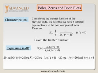
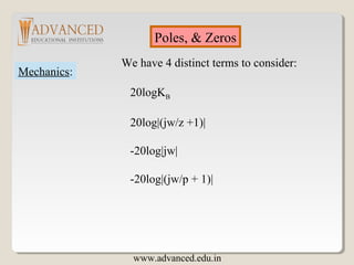
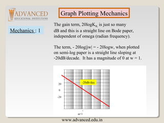
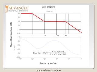
The document discusses Bode plots, which are frequency domain techniques used to analyze linear time-invariant systems. It covers poles and zeros, transfer functions, the S-plane, mechanics for constructing Bode plots, examples of plotting Bode plots by hand and using MATLAB, and designing a system to meet a target Bode plot specification. Key steps include identifying poles and zeros, approximating plots between break frequencies, and using MATLAB tools like Bode and Simulink to validate designs.

1. www.advanced.edu.in
BODE PLOT
By: Shalini Singh
Assistant Professor

2. CONTENTS
• Introduction
•Poles & Zeros
•Transfer Function
•S-Plane
•Mechanism For Solving Bode Plot
•Examples
•Graph Plotting
•Bode Plot Using MATLAB
•Simulink Model & Graph
www.advanced.edu.in

3. www.advanced.edu.in
INTRODUCTION
Bode Plot is a frequency domain technique in which magnitude &
phase are drawn one below the other .
• Graph I – The magnitude (M) of the Transfer Function &
• Graph II – The Phase angle ( ) as function of frequency (ɸ ω)

4. Poles and Zeros and Transfer Functions
Transfer
Function:
A transfer function is defined as the ratio of the
Laplace
transform of the output to the input with all initial
conditions equal to zero. Transfer functions are
defined
only for linear time invariant systems.Considerations: Transfer functions can usually be expressed as the
ratio
of two polynomials in the complex variable, s.
Factorization: A transfer function can be factored into the following
form.
)(...))((
)(...))((
)(
21
21
n
m
pspsps
zszszsK
sG
+++
+++
=
The roots of the numerator polynomial are called zeros.
The roots of the denominator polynomial are called poles.
www.advanced.edu.in

5. Poles, Zeros and the S-Plane
An Example:
You are given the following transfer function. Show the
poles and zeros in the s-plane.
)10)(4(
)14)(8(
)(
++
++
=
sss
ss
sG
S - plane
xxoxo
0-4-8-10-14
origin
σ axis
jω axis
www.advanced.edu.in

6. Poles, Zeros and Bode Plots
Characterization: Considering the transfer function of the
previous slide. We note that we have 4 different
types of terms in the previous general form:
These are:
)1/(,
)1/(
1
,
1
, +
+
zs
pss
KB
Expressing in dB:
Given the tranfer function:
)1/)((
)1/(
)(
+
+
=
pjwjw
zjwK
jwG B
|1/|log20||log20|)1/(|log20log20|(|log20 +−−++= pjwjwzjwKjwG B
www.advanced.edu.in

7. Poles, & Zeros
Mechanics:
We have 4 distinct terms to consider:
20logKB
20log|(jw/z +1)|
-20log|jw|
-20log|(jw/p + 1)|
www.advanced.edu.in

8. Graph Plotting Mechanics
Mechanics : 1
The gain term, 20logKB, is just so many
dB and this is a straight line on Bode paper,
independent of omega (radian frequency).
The term, - 20log|jw| = - 20logw, when plotted
on semi-log paper is a straight line sloping at
-20dB/decade. It has a magnitude of 0 at w = 1.
0
20
-20
ω=1
-20db/dec
www.advanced.edu.in

9. Mechanics: 2
The term, - 20log|(jw/p + 1), is drawn with the
following approximation: If w < p we use the
approximation that –20log|(jw/p + 1 )| = 0 dB,
a flat line on the Bode. If w > p we use the
approximation of –20log(w/p), which slopes at
-20dB/dec starting at w = p. Illustrated below.
It is easy to show that the plot has an error of
-3dB at w = p and – 1 dB at w = p/2 and w = 2p.
One can easily make these corrections if it is
appropriate.
0
20
-20
-40
-20db/dec
www.advanced.edu.in

10. 0
20
-20
-40
ω = z
+20db/dec
Mechanics: 3
When we have a term of 20log|(jw/z + 1)| we
approximate it be a straight line of slop 0 dB/dec
when w < z. We approximate it as 20log(w/z)
when w > z, which is a straight line on Bode paper
with a slope of + 20dB/dec. Illustrated below.
www.advanced.edu.in

11. Example 1:
Given: 50,000( 10)
( )
( 1)( 500)
jw
G jw
jw jw
+
=
+ +
First: Always, always, always get the poles and zeros in a form such that
the constants are associated with the jw terms. In the above example
we do this by factoring out the 10 in the numerator and the 500 in the
denominator.
50,000 10( /10 1) 100( /10 1)
( )
500( 1)( / 500 1) ( 1)( / 500 1)
x jw jw
G jw
jw jw jw jw
+ +
= =
+ + + +
Second: When you have neither poles nor zeros at 0, start the Bode
at 20log10K = 20log10100 = 40 dB in this case.
www.advanced.edu.in

12. Third: Observe the order in which the poles and zeros occur.
This is the secret of being able to quickly sketch the Bode.
In this example we first have a pole occurring at 1 which
causes the Bode to break at 1 and slope – 20 dB/dec.
Next, we see a zero occurs at 10 and this causes a
slope of +20 dB/dec which cancels out the – 20 dB/dec,
resulting in a flat line ( 0 db/dec). Finally, we have a
pole that occurs at w = 500 which causes the Bode
to slope down at – 20 dB/dec.
We are now ready to draw the Bode.
Before we draw the Bode we should observe the range
over which the transfer function has active poles and zeros.
This determines the scale we pick for the w (rad/sec)
at the bottom of the Bode.
The dB scale depends on the magnitude of the plot and
experience is the best teacher here.
www.advanced.edu.in

13. dB Mag
Bode Plot Magnitude for 100(1+jw/10)/(1Bode Plot Magnitude for 100(1+jw/10)/(1
+ jw/1)(1 + jw/500)+ jw/1)(1 + jw/500)
ω (rad/sec)
Phase (deg)0
20
40
-20
-60
-60
0.1 1 10 100 1000 10000
www.advanced.edu.in

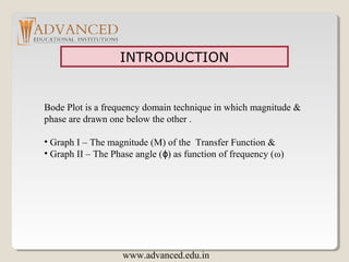
14. Using Matlab For Frequency Response
Instruction:
We can use Matlab to run the frequency response for
the previous example. We place the transfer function
in the form:
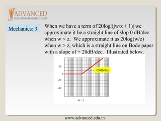
]500501[
]500005000[
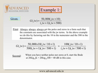
)500)(1(
)10(5000
2
++
+
=
++
+
ss
s
ss
s
The Matlab Program
num = [5000 50000];
den = [1 501 500];
Bode (num, den)
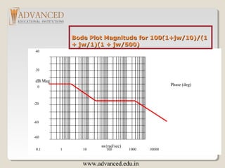
In the following slide, the resulting magnitude and phase plots (exact)
are shown in light color (blue). The approximate plot for the magnitude
(Bode) is shown in heavy lines (red). We see the 3 dB errors at the
corner frequencies.
www.advanced.edu.in

15. Frequency (rad/sec)
Phase(deg);Magnitude(dB)
Bode Diagrams
-10
0
10
20
30
40
From: U(1)
10-1
100
101
102
103
104
-100
-80
-60
-40
-20
0
To:Y(1)
1 10 100 500
)500/1)(1(
)10/1(100
)(
jwjw
jw
jwG
++
+
=Bode for:
www.advanced.edu.in

16. Phase Plots for Bode
Comment:
Generally, the phase for a Bode plot is not as easy to draw
or approximate as the magnitude. In this course we will use
an analytical method for determining the phase if we want to
make a sketch of the phase.
Illustration:
Consider the transfer function of the previous
example.
We express the angle as follows:
)500/(tan)1/(tan)10/(tan)( 111
wwwjwG −−−
−−=∠
We are essentially taking the angle of each pole and zero.
Each of these are expressed as the tan-1
(j part/real part)
Usually, about 10 to 15 calculations are sufficient to determine
a good idea of what is happening to the phase.
www.advanced.edu.in

17. Bode Plots
Example 1: Given the transfer function. Plot the Bode magnitude.
2
)100/1(
)10/1(100
)(
ss
s
sG
+
+
=
Consider first only the two terms of jw
100
Which, when expressed in dB, are; 20log100 – 20 logw.
This is plotted below.
0
20
40
-20
The is
a tentative line we use
until we encounter the
first pole(s) or zero(s)
not at the origin.
-20db/dec
www.advanced.edu.in
ω (rad/sec)

18. ω (rad/sec)
dB Mag Phase (deg)
0
20
40
60
-20
-40
-60
1 10 100 10000.1
2
)100/1(
)10/1(100
)(
ss
s
sG
+
+
=
ω (rad/sec)
dB Mag Phase (deg)
0
20
40
60
-20
-40
-60
1 10 100 10000.1
-20db/dec
-40 db/dec
2
)100/1(
)10/1(100
)(
ss
s
sG
+
+
=
The completed plot is shown below.

19. Design Problem: Design a G(s) that has the following Bode plot.
dB mag
ω rad/sec
0
20
40
0.1 1 10 100 1000
30 900
30 dB
+40 dB/dec
-40dB/dec
? ?
Example 1:

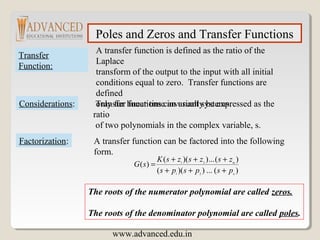
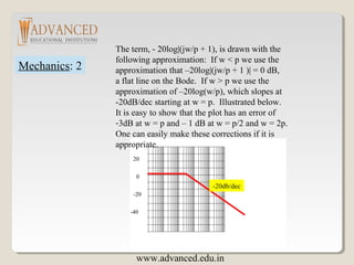
20. Procedure for desgining
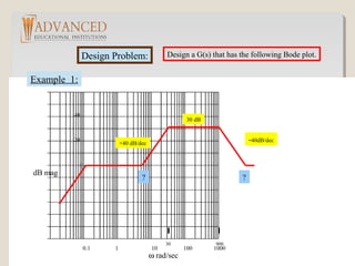
Procedure: The two break frequencies need to be found.
Recall:
#dec = log10[w2/w1]
Then we have:
(#dec)( 40dB/dec) = 30 dB
log10[w1/30] = 0.75 w1 = 5.33 rad/sec
Also: log10[w2/900] (-40dB/dec) = - 30dB
This gives w2 = 5060 rad/sec
www.advanced.edu.in

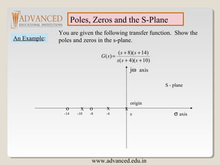
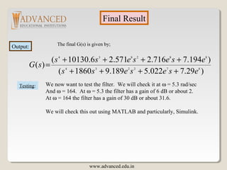
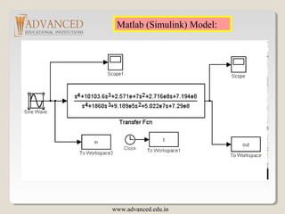
21. Steps
2 2
2 2
(1 / 5.3) (1 / 5060)
( )
(1 / 30) (1 / 900)
s s
G s
s s
+ +
=
+ +
Clearing: 2 2
2 2
( 5.3) ( 5060)
( )
( 30) ( 900)
s s
G s
s s
+ +
=
+ +
Use Matlab and conv:
2 2 7
1 ( 10.6 28.1) 2 ( 10120 2.56 )N s s N s s xe= + + = + +
N = conv(N1,N2)
N1 = [1 10.6 28.1] N2 = [1 10120 2.56e+7]
1 1.86e+3 2.58e+7 2.73e+8 7.222e+8
s4
s3
s2
s1
s0
www.advanced.edu.in

22. Final Result
Output: The final G(s) is given by;
Testing: We now want to test the filter. We will check it at ω = 5.3 rad/sec
And ω = 164. At ω = 5.3 the filter has a gain of 6 dB or about 2.
At ω = 164 the filter has a gain of 30 dB or about 31.6.
We will check this out using MATLAB and particularly, Simulink.
)29.7022.5189.91860(
)194.7716.2571.26.10130(
)( 872234
882834
esesess
esesess
sG
++++
++++
=
www.advanced.edu.in

23. Matlab (Simulink) Model:
www.advanced.edu.in

24. Scope 1 Response at ω = 5.3 rad/sec
Simulink Graph
www.advanced.edu.in
Matlab (Simulink) Model: Conclusion

25. Scope 2 Output at ω = 70 rad/sec
Simulink Graph
www.advanced.edu.in

26. Shalini Singh
ASSISTANT PROFESSOR
shalinisingh1344@gmail.com
Advanced Educational Institutions
70 km Milestone,
Delhi-Mathura Road, Dist. Palwal,
Haryana-121105
Enquiry No: +91–1275–398400, 302222
Tele Fax: +91-1275-398406
E-mail: info@advancedinstitutions.com
Website: www.advanced.edu.in
www.advanced.edu.in