1) The document discusses system models using differential equations to describe dynamic systems. Differential equations can model both mechanical and electrical systems.
2) Translational and rotational systems involving springs, dampers, masses and inertias can be modeled using differential equations relating forces, torques, positions, velocities and accelerations.
3) The document provides examples of differential equation models for various mechanical systems like masses on springs, pendulums and mass-spring-damper systems. It also discusses modeling concepts like linearization and Laplace transforms.
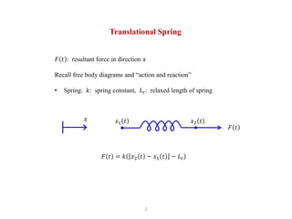
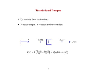
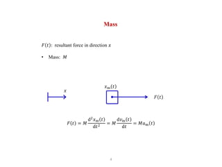
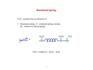
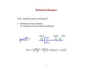
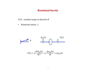
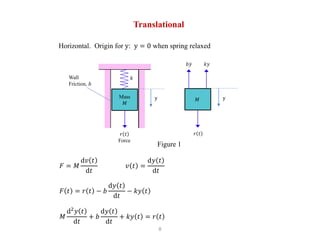
Power series convergence ,taylor & laurent's theoremPARIKH HARSHIL
This ppt clear your concept about Power series - Convergence & give overview about Taylor & Laurent's Theorem . This is very Helpfull for CVNM subject of GTU
Power series convergence ,taylor & laurent's theoremPARIKH HARSHIL
This ppt clear your concept about Power series - Convergence & give overview about Taylor & Laurent's Theorem . This is very Helpfull for CVNM subject of GTU
Generally it has been noticed that differential equation is solved typically. The Laplace transformation makes it easy to solve. The Laplace transformation is applied in different areas of science, engineering and technology. The Laplace transformation is applicable in so many fields. Laplace transformation is used in solving the time domain function by converting it into frequency domain. Laplace transformation makes it easier to solve the problems in engineering applications and makes differential equations simple to solve. In this paper we will discuss how to follow convolution theorem holds the Commutative property, Associative Property and Distributive Property. Dr. Dinesh Verma"Application of Convolution Theorem" Published in International Journal of Trend in Scientific Research and Development (ijtsrd), ISSN: 2456-6470, Volume-2 | Issue-4 , June 2018, URL: http://www.ijtsrd.com/papers/ijtsrd14172.pdf http://www.ijtsrd.com/mathemetics/applied-mathamatics/14172/application-of-convolution-theorem/dr-dinesh-verma
Stability: Methods of determining stability, Routh Hurwitz Criterion, Root Locus, Frequency Domain Analysis: Resonant Peak, Resonant frequency and Bandwidth of the second order system, Effect of adding a zero and a pole to the forward path, Nyquist Stability Criterion, Relative Stability: Gain Margin and Phase Margin, Bode Plot.
MTH101 - Calculus and Analytical Geometry- Lecture 44Bilal Ahmed
Virtual University
Course MTH101 - Calculus and Analytical Geometry
Lecture No 44
Instructor's Name: Dr. Faisal Shah Khan
Course Email: mth101@vu.edu.pk
power series is the chapter of complex variable and numeric methods.
topics covered are
singular point and its classifications
residue theorem
rouche's theorem
In this slide i am trying my best to describe about the power series. If you face any problem or anything that you can't understand please contact me on facebook:https://www.facebook.com/asadujjaman.asad.79
z-Transform is for the analysis and synthesis of discrete-time control systems.The z transform in discrete-time systems play a similar role as the Laplace transform in continuous-time systems
نموذج الدراسة :
Effect of convective conditions in a radiative peristaltic flow of pseudoplastic nanofluid through a porous medium in a tapered an inclined asymmetric channel
تأثير الشروط الحدودية على الجريان الشعاعي للمائع النانوي الكاذب خلال وسط مسامي في قناة مستدقة مائلة غير متماثلة
Elasticity, Plasticity and elastic plastic analysisJAGARANCHAKMA2
It is actually the basis of structural engineering to study elasticity and plasticity analysis. So people who are also studying in various fields of structure and need to analyze finite element analysis also need to study this basis.
Safalta Digital marketing institute in Noida, provide complete applications that encompass a huge range of virtual advertising and marketing additives, which includes search engine optimization, virtual communication advertising, pay-per-click on marketing, content material advertising, internet analytics, and greater. These university courses are designed for students who possess a comprehensive understanding of virtual marketing strategies and attributes.Safalta Digital Marketing Institute in Noida is a first choice for young individuals or students who are looking to start their careers in the field of digital advertising. The institute gives specialized courses designed and certification.
for beginners, providing thorough training in areas such as SEO, digital communication marketing, and PPC training in Noida. After finishing the program, students receive the certifications recognised by top different universitie, setting a strong foundation for a successful career in digital marketing.
This slide is special for master students (MIBS & MIFB) in UUM. Also useful for readers who are interested in the topic of contemporary Islamic banking.
Delivering Micro-Credentials in Technical and Vocational Education and TrainingAG2 Design
Explore how micro-credentials are transforming Technical and Vocational Education and Training (TVET) with this comprehensive slide deck. Discover what micro-credentials are, their importance in TVET, the advantages they offer, and the insights from industry experts. Additionally, learn about the top software applications available for creating and managing micro-credentials. This presentation also includes valuable resources and a discussion on the future of these specialised certifications.
For more detailed information on delivering micro-credentials in TVET, visit this https://tvettrainer.com/delivering-micro-credentials-in-tvet/
Macroeconomics- Movie Location
This will be used as part of your Personal Professional Portfolio once graded.
Objective:
Prepare a presentation or a paper using research, basic comparative analysis, data organization and application of economic information. You will make an informed assessment of an economic climate outside of the United States to accomplish an entertainment industry objective.
Unit 8 - Information and Communication Technology (Paper I).pdfThiyagu K
This slides describes the basic concepts of ICT, basics of Email, Emerging Technology and Digital Initiatives in Education. This presentations aligns with the UGC Paper I syllabus.
This presentation includes basic of PCOS their pathology and treatment and also Ayurveda correlation of PCOS and Ayurvedic line of treatment mentioned in classics.
Biological screening of herbal drugs: Introduction and Need for
Phyto-Pharmacological Screening, New Strategies for evaluating
Natural Products, In vitro evaluation techniques for Antioxidants, Antimicrobial and Anticancer drugs. In vivo evaluation techniques
for Anti-inflammatory, Antiulcer, Anticancer, Wound healing, Antidiabetic, Hepatoprotective, Cardio protective, Diuretics and
Antifertility, Toxicity studies as per OECD guidelines
Thinking of getting a dog? Be aware that breeds like Pit Bulls, Rottweilers, and German Shepherds can be loyal and dangerous. Proper training and socialization are crucial to preventing aggressive behaviors. Ensure safety by understanding their needs and always supervising interactions. Stay safe, and enjoy your furry friends!
Lecture Notes: EEEC4340318 Instrumentation and Control Systems - System Models
1. EEEC4340318 INSTRUMENTATION AND CONTROL SYSTEMS
System Models
FACULTY OF ENGINEERING AND COMPUTER TECHNOLOGY
DIPLOMA IN ELECTRICALAND ELECTRONIC ENGINEERING
Ravandran Muttiah BEng (Hons) MSc MIET
2. 1
Differential Equation Models
• Most of the systems that we will deal with are dynamic
• Differential equations provide a powerful way to describe
dynamic systems
• Will form the basis of our models
• We saw differential equations for inductors and capacitors.
• What about mechanical systems?
both translational and rotational
3. 2
Translational Spring
𝐹 𝑡 : resultant force in direction 𝑥
Recall free body diagrams and “action and reaction”
• Spring. 𝑘: spring constant, 𝐿r: relaxed length of spring
𝐹 𝑡 = 𝑘 𝑥2 𝑡 − 𝑥1 𝑡 − 𝐿r
𝑥 𝑥1 𝑡 𝑥2 𝑡
𝐹 𝑡
11. 10
• Nature does not have many linear systems.
• However, many systems behave approximately linearly in the
neighbourhood of a given point.
• Apply first-order Taylor’s Series at a given point.
• Obtain a locally linear model.
• In this course we will focus on the case of a single linearized
differential equation model for the system, in which the
coefficients are constants.
• e.g., in previous examples mass, viscosity and spring constant
did not change with time, position, velocity, temperature, etc.
Taylor’s Series
12. 11
Pendulum Example
Assume shaft is light with respect to 𝑀, and stiff with respect to
gravitational forces.
Torque due to gravity: 𝑇 𝜃 = 𝑀𝑔𝐿 sin 𝜃
Apply Taylor’s series around 𝜃 = 0:
𝑇 𝜃 = 𝑀𝑔𝐿 𝜃 −
𝜃3
3!
+
𝜃5
5!
−
𝜃7
7!
+ ⋯
For small 𝜃 around 𝜃 = 0 we can build an approximate model that
is linear,
𝑇 𝜃 ≈ 𝑀𝑔𝐿𝜃
14. 13
Laplace Transform
Once we have a linearised differential equation (with constant
coefficients) we can take Laplace Transforms to obtain the transfer
function.
We will consider the “one-sided” Laplace transform, for signals
that are zero to the left of the origin.
𝐹 𝑠 =
0−
∞
𝑓 𝑡 e−𝑠𝑡
d𝑡
What does
∞
mean ? lim𝑇→∞
𝑇
.
Does this limit exist ?
If 𝑓 𝑡 < 𝑀e𝛼𝑡
, then exists for all Re 𝑠 > 𝛼.
Includes all physically realisable signals.
Note: When multiplying transfer function by Laplace of input,
output is only valid for values of 𝑠 in intersection of regions of
convergence.
15. 14
Poles And Zeros
In this course, most Laplace transforms will be rational functions,
that is, a ratio of two polynomials in 𝑠; i.e.,
𝐹 𝑠 =
𝑛F 𝑠
𝑑F 𝑠
where 𝑛F 𝑠 and 𝑑F 𝑠 are polynomials.
Definitions:
- Poles of 𝐹 𝑠 are the roots of 𝑑F 𝑠
- Zeros of 𝐹 𝑠 are the roots of 𝑛F 𝑠
Hence,
𝐹 𝑠 =
𝐾F 𝑖=1
𝑀
𝑠 + 𝑧𝑖
𝑗=1
𝑛
𝑠 + 𝑝𝑗
=
𝐾F 𝑖=1
𝑀
𝑧𝑖
𝑗=1
𝑛
𝑝𝑗
𝑖=1
𝑀 𝑠
𝑧𝑖 + 1
𝑗=1
𝑛 𝑠
𝑝𝑗 + 1
where −𝑧𝑖 are the zeros and −𝑝𝑗 are the poles.
16. 15
Visualising Poles And Zeros
Consider the simple Laplace transform 𝐹 𝑠 =
𝑠 𝑠+3
𝑠2+2𝑠+5
zeros: 0, −3; poles: −1 + j2, −1 − j2
Figure 4: Pole-zero plot (left) and magnitude of 𝐹 𝑠 right
17. 16
𝐹 𝑠 from above (left) and previous view of 𝐹 𝑠 right.
Figure 5
18. 17
Laplace Transforms Pairs
Simple ones can be computed analytically;
For more complicated ones, one can typically obtain the inverse
Laplace transform by:
- Identifying poles;
- Constructing partial fraction expansion;
- Using of properties and some simple pairs to invent each
component of partial fraction expansion.
21. 20
Final Value Theorem
Can we avoid having to do an inverse Laplace transform ?
Sometimes.
Consider the case when we only want to find the final value of
𝑓 𝑡 , namely lim𝑡→∞𝑓 𝑡 .
If 𝐹 𝑠 has all its poles in the left half plane, except, perhaps, for a
single pole at the origin, then,
lim
𝑡→∞
𝑓 𝑡 = lim
𝑠→0
𝑠𝐹 𝑠
Common application: Steady state value of step response.
What if there are poles in Right Half Plane (RHP), or on the j𝜔 -
axis and not at the origin ?
22. 21
Mass-Spring-Damper System
Horizontal (no gravity)
Set origin of 𝑦 where spring is “relaxed”
𝐹 = 𝑀
d𝑣 𝑡
d𝑡
𝑣 𝑡 =
d𝑦 𝑡
d𝑡
𝐹 𝑡 = 𝑟 𝑡 − 𝑏
d𝑦 𝑡
d𝑡
− 𝑘𝑦 𝑡 𝑀
d2
𝑦 𝑡
d𝑡
+ 𝑏
d𝑦 𝑡
d𝑡
+ 𝑘𝑦 𝑡 = 𝑟 𝑡
Mass
𝑀
Wall
Friction, 𝑏
y
𝑘
𝑟 𝑡
Force
𝑀
𝑘𝑦
𝑏𝑦
𝑟 𝑡
y
Figure 7
24. 23
Response To Static Initial Condition
Spring stretched to a point 𝑦0, held, then let go at time 𝑡 = 0
Hence, 𝑟 𝑡 = 0 and
d𝑦 𝑡
d𝑡 𝑡=0
= 0
Hence,
𝑌 𝑠 =
𝑠 +
𝑏
𝑀
𝑠2 +
𝑏
𝑀
𝑠 +
𝑘
𝑀
𝑦0
What can we learn about this response without having to invert 𝑌 𝑠
29. 28
Define 𝜎 = 𝜁𝜔𝑛, 𝜔d = 𝜔𝑛 1 − 𝜁2. Response is:
𝑦 𝑡 = 𝑐1e−𝜎𝑡
cos 𝜔d𝑡 + 𝑐2e−𝜎𝑡
sin 𝜔d𝑡
= 𝐴e−𝜎𝑡
cos 𝜔d𝑡 + 𝜙
Homework: Relate 𝐴 and 𝜙 to 𝑐1 and 𝑐2.
Homework: Write the initial conditions 𝑦 0 = 𝑦0 and
d𝑦 𝑡
d𝑥 𝑡=0
= 0 in terms of 𝑐1 and 𝑐2, and in terms of 𝐴 and 𝜙
45. 44
Transfer Function
Definition:
Laplace transform of output over Laplace transform of input when
initial conditions are zero.
Most of the transfer functions in this course will be ratios of
polynomials in 𝑠.
Hence, poles and zeros of transfer functions have natural definitions.
Example:
Recall the mass-spring-damper system,
47. 46
Step Response
Recall that 𝑢 𝑡 ↔
1
𝑠
Therefore, for transfer function 𝐺 𝑠 , the step response is:
ℒ−1
𝐺 𝑠
𝑠
For the mass-spring-damper system, step response is,
ℒ−1
1
𝑠 𝑀𝑠2 + 𝑏𝑠 + 𝑘
What is the final position for a step input ?
Recall final value theorem. Final position is
1
𝐾
.
What about the complete step response ?
48. 47
Step response:
ℒ−1
𝐺 𝑠
1
𝑠
Hence poles of Laplace transform of step response are poles of 𝐺 𝑠 ,
plus an additional pole at 𝑠 = 0.
For the mass-spring-damper system, using partial fractions, step
response is:
ℒ−1
1
𝑠 𝑀𝑠2 + 𝑏𝑠 + 𝑘
= ℒ−1
1
𝑘
𝑠
−
1
𝑘
ℒ−1
𝑀𝑠 + 𝑏
𝑀𝑠2 + 𝑏𝑠 + 𝑘
=
1
𝑘
𝑢 𝑡 −
1
𝑘
ℒ−1
𝑀𝑠 + 𝑏
𝑀𝑠2 + 𝑏𝑠 + 𝑘
Consider again the case of 𝑀 = 𝑘 = 1, 𝑏 = 3 → 0.
𝜔𝑛 = 1, 𝜁 = 1.5 → 0.
63. 62
We will consider linearised model for each component.
Flux in the air gap: ∅ 𝑡 = 𝐾f𝑖f 𝑡
Torque: 𝑇m 𝑡 = 𝐾1∅ 𝑡 𝑖a 𝑡 = 𝐾1𝐾f𝑖f 𝑡 𝑖a 𝑡
Is that linear ? Only if one of 𝑖f 𝑡 or 𝑖f 𝑡 is constant.
We will consider “armature control”: 𝑖f 𝑡 constant.
A DC Motor
Figure 9
64. 63
Armature Controlled DC Motor
𝑖f 𝑡 will be constant (to set up magnetic field), 𝑖f 𝑡 = 𝐼f
Torque: 𝑇m 𝑡 = 𝐾1𝐾f𝐼f𝑖a 𝑡 = 𝐾m𝑖a 𝑡
Will control motor using armature voltage 𝑉
a 𝑡 .
What is the transfer function from 𝑉
a 𝑠 to angular position 𝜃 𝑠 ?
Origin ?
65. 64
𝑇m 𝑡 = 𝐾m𝑖a 𝑡 ↔ 𝑇m 𝑠 = 𝐾m𝐼a 𝑠
Kirchhoff Voltage Law: 𝑉
a 𝑠 = 𝑅a + 𝑠𝐿a 𝐼a 𝑠 + 𝑉b 𝑠
𝑉b 𝑠 is back-emf voltage, due to Faraday’s Law.
𝑉b 𝑠 = 𝐾b𝜔 𝑠 ,
where 𝜔 𝑠 = 𝑠𝜃 𝑠 is rotational velocity.
Remember: transfer function implies zero initial conditions.
Towards Transfer Function
66. 65
Torque on load: 𝑇L 𝑠 = 𝑇m 𝑠 − 𝑇d 𝑠
𝑇d 𝑠 : disturbance. Often small, unknown.
Load torque and load angle (Newton plus friction):
𝑇L 𝑠 = 𝐽𝑠2
𝜃 𝑠 + 𝑏𝑠𝜃 𝑠
Now put it all together.
68. 67
Transfer Function
𝐾m
𝑅a + 𝐿a𝑠
Armature
1
𝐽𝑠 + 𝑏
1
𝑠
𝐾b
Disturbance
𝑇d 𝑠
Position
𝜃 𝑠
𝑉
a 𝑠
+
−
+
−
𝑇m 𝑠 𝑇L 𝑠
Speed
𝜔 𝑠
Back Electromotive Force
Set 𝑇d 𝑠 = 0 and solve (you MUST do this yourself)
𝐺 𝑠 =
𝜃 𝑠
𝑉
a 𝑠
=
𝐾m
𝑠 𝑅a + 𝑠𝐿a 𝐽𝑠 + 𝑏 + 𝐾b𝐾m
=
𝐾m
𝑠 𝑠2 + 2𝜁𝜔𝑛𝑠 + 𝜔𝑛
2
Figure 10
69. 68
Second Order Approximation
𝐺 𝑠 =
𝜃 𝑠
𝑉
a 𝑠
=
𝐾m
𝑠 𝑅a + 𝑠𝐿a 𝐽𝑠 + 𝑏 + 𝐾b𝐾m
Sometimes armature time constant, 𝜏𝑎 =
𝐿a
𝑅a
is negligible
Hence (you MUST derive this yourself)
𝐺 𝑠 ≈
𝐾m
𝑠 𝑅a 𝐽𝑠 + 𝑏 𝐾b𝐾m
=
𝐾𝑚
𝑅a𝑏 + 𝐾b𝐾m
𝑠 𝜏1𝑠 + 1
where 𝜏1 =
𝑅a𝐽
𝑅a𝑏+𝐾b𝐾m
70. 69
Model For A Disk Drive Read System
Uses a permanent magnet DC motor
Can be modelled using armature control model with 𝐾b = 0
Hence, motor transfer function:
𝐺 𝑠 =
𝜃 𝑠
𝑉
a 𝑠
=
𝐾m
𝑠 𝑅a + 𝑠𝐿a 𝐽𝑠 + 𝑏
Assume for now that the arm is stiff.
Figure 11
71. 70
Typical Values
Parameter Symbol Typical Value
Inertia of Arm and Read Head 𝐽 1 Nm𝑠2
/rad
Friction 𝑏 20 Nms/rad
Amplifier 𝐾a 10-1000
Armature Resistance 𝑅 1 Ω
Motor Constant 𝐾m 5 Nm/A
Armature Inductance 𝐿 1 mH
𝐺 𝑠 =
5000
𝑠 𝑠 + 20 𝑠 + 1000
Table 1
72. 71
Time Constants
Initial model,
𝐺 𝑠 =
5000
𝑠 𝑠 + 20 𝑠 + 1000
Motor time constant =
1
20
= 50 ms
Armature time constant =
1
1000
= 1 ms
Hence,
𝐺 𝑠 ≈ 𝐺 𝑠 =
5
𝑠 𝑠 + 20
73. 72
A Simple Feedback Controller
Now that we have a model, how to control ?
Simple idea: Apply voltage to motor that is proportional to error
between where we are and where we want to be.
Amplifier
Control Device Actuator and Read Arm
Input
Voltage Actual
Head
Position
+
−
DC Motor and Arm
Sensor
Read Head and Index Track on Disk
Desired
Head
Position
Error
Figure 12
74. 73
𝐾a
Amplifier Motor and Arm 𝐺 𝑠
𝑉 𝑠
𝑌 𝑠
+
−
𝐺 𝑠 =
𝐾m
𝑠 𝐽𝑠 + 𝑏 𝐿𝑠 + 𝑅
Sensor
𝐻 𝑠 = 1
𝑅 𝑠
𝐸 𝑠
Here, 𝑉 𝑠 = 𝑉
a 𝑠 and 𝑌 𝑠 = 𝜃 𝑠
Figure 13
75. 74
Simplified Block Diagram
𝐾a 𝑌 𝑠
+
−
𝐺 𝑠
𝑅 𝑠
What is the transfer function from command to position ? Derive this
yourself.
𝑌 𝑠
𝑅 𝑠
=
𝐾a𝐺 𝑠
1 + 𝐾a𝐺 𝑠
Using second-order approximation, 𝐺 𝑠 ≈ 𝐺 𝑠 =
5
𝑠 𝑠+20
𝑌 𝑠 ≈
5𝐾a
𝑠2 + 20𝑠 + 5𝐾a
𝑅 𝑠
For 0 < 𝐾a < 20: overdamped
For 𝐾a > 20: underdamped
Figure 14
76. 75
Response To 𝒓 𝒕 = 𝟎. 𝟏𝒖 𝒕 ; 𝑲𝐚 = 𝟏𝟎
Slow. Slower than IBMs first drive from late 1950’s.
Disks in the 1970’s had 25 ms seek times; now < 10 ms
Perhaps increase 𝐾a ?
That would result in a “bigger” input to the motor for a given error.
Poles in s-plane Response
77. 76
Response To 𝒓 𝒕 = 𝟎. 𝟏𝒖 𝒕 ; 𝑲𝐚 = 𝟏𝟎, 𝟏𝟓
Poles in s-plane Response
Changing 𝐾a changes the position of the closed loop poles.
Hence, step response changes.
78. 77
Response To 𝒓 𝒕 = 𝟎. 𝟏𝒖 𝒕 ; 𝑲𝐚 = 𝟏𝟎, 𝟏𝟓, 𝟐𝟎
Changing 𝐾a changes the position of the closed loop poles.
Hence, step response changes (now critically damped).
79. 78
Response To 𝒓 𝒕 = 𝟎. 𝟏𝒖 𝒕 ; 𝑲𝐚 = 𝟏𝟎, 𝟏𝟓, 𝟐𝟎, 𝟒𝟎
Changing 𝐾a changes the position of the closed loop poles.
Hence, step response changes (now underdamped).
80. 79
Response To 𝒓 𝒕 = 𝟎. 𝟏𝒖 𝒕 ; 𝑲𝐚 = 𝟏𝟎, 𝟏𝟓, 𝟐𝟎, 𝟒𝟎, 𝟔𝟎
Changing 𝐾a changes the position of the closed loop poles.
Hence, step response changes (now more underdamped).
81. 80
Response To 𝒓 𝒕 = 𝟎. 𝟏𝒖 𝒕 ; 𝑲𝐚 = 𝟏𝟎, 𝟏𝟓, 𝟐𝟎, 𝟒𝟎, 𝟔𝟎, 𝟖𝟎
What is happening to the settling time of the underdamped cases ?
Only just beats IBM’s first drive.
What else could we do with the controller ? Prediction ?
82. 81
Block Diagram Models
As we have just seen, a convenient way to represent a transfer function is via
a block diagram.
In this case, 𝑈 𝑠 = 𝐺c 𝑠 𝑅 𝑠 and 𝑌 𝑠 = 𝐺 𝑠 𝑈 𝑠
Hence, 𝑌 𝑠 = 𝐺 𝑠 𝐺c 𝑠 𝑅 𝑠
Consistent with the engineering procedure of breaking things up into little
bits, studying the little bits, and then put them together.
𝐺c 𝑠 𝑌 𝑠
𝐺 𝑠
𝑅 𝑠
Figure 15
Controller Process
𝑈 𝑠
84. 83
Example: Loop Transfer Function
𝐺c 𝑠
Controller
𝑍 𝑠
𝑌 𝑠
+
−
𝑅 𝑠
𝐸a 𝑠
Figure 17
𝐺a 𝑠
Actuator
𝐺 𝑠
Process
𝐻 𝑠
Sensor
𝑈 𝑠
𝐵 𝑠
𝐸𝑎 𝑠 = 𝑅 𝑠 − 𝐵 𝑠 = 𝑅 𝑠 − 𝐻 𝑠 𝑌 𝑠
𝑌 𝑠 = 𝐺 𝑠 𝑈 𝑠 = 𝐺 𝑠 𝐺a 𝑠 𝑍 𝑠 = 𝐺 𝑠 𝐺a 𝑠 𝐺c 𝑠 𝐸a 𝑠
= 𝐺 𝑠 𝐺a 𝑠 𝐺c 𝑠 𝑅 𝑠 − 𝐻 𝑠 𝑌 𝑠
𝑌 𝑠
𝑅 𝑠
=
𝐺 𝑠 𝐺a 𝑠 𝐺c 𝑠
1 + 𝐺 𝑠 𝐺𝑎 𝑠 𝐺𝑐 𝑠 𝐻 𝑠
Each transfer function is a ratio of polynomials in 𝑠.
What is
𝐸a 𝑠
𝑅 𝑠
?
85. 84
Block Diagram Transformations
Combining Block In Cascade
Original Diagram Equivalent Diagram
𝐺1 𝑠
𝑋1 𝐺2 𝑠 𝑋3
𝑋2
𝐺1𝐺2
𝑋1 𝑋3
Moving A Summing Point Behind A Block
𝐺 𝑋3
+
±
𝑋1
𝑋2
𝐺
+
±
𝑋1
𝑋2
𝐺
𝑋3
Original Diagram Equivalent Diagram
86. 85
Moving A Pickoff Point Ahead Of A Block
Original Diagram Equivalent Diagram
𝐺
𝑋1 𝑋2 𝐺
𝑋1 𝑋3
Moving A Pickoff Point Behind A Block
𝐺
𝑋1
1
𝐺
𝑋2
Original Diagram Equivalent Diagram
𝑋2
𝐺
𝑋2
𝐺
𝑋1 𝑋2
𝑋1
𝑋1
87. 86
Moving A Summing Point Ahead Of A Block
Original Diagram Equivalent Diagram
𝐺
𝑋1 𝑋3 𝐺 𝑋3
Eliminating A Feedback Loop
𝐺
1 ± 𝐺𝐻
𝑋1
𝑋2
Original Diagram Equivalent Diagram
𝑋2
1
𝐺
𝑋2
+
± ±
𝑋1
+
𝐺 𝑋2
𝐻
±
𝑋1
+