

![Creating / Acquiring Some Signals
• Task 1.1 - Other signals?
– Text Format
• MATLAB can load a list of numbers very easily through the
command “load”
• Start “Notepad”, enter a coma separated list of
numbers, save the file in your current path, load the file in
MATLAB.
– WAV Format
• Sound files can be acquired from “freesound.org” and be
loaded into your workspace through “wavread”
• Locate a .wav file, load it into matlab using
[x7, Fs]=wavread(‘path/to/some/file.wav’);](https://image.slidesharecdn.com/aafftspect-120308063056-phpapp01/85/The-FFT-And-Spectral-Analysis-28-320.jpg)


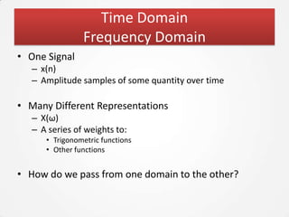
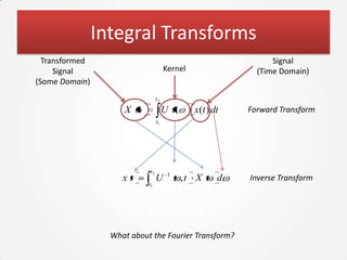
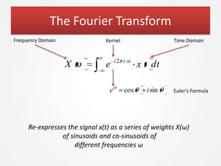
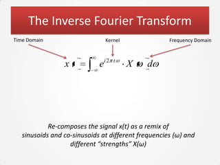
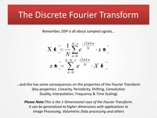
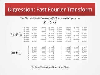
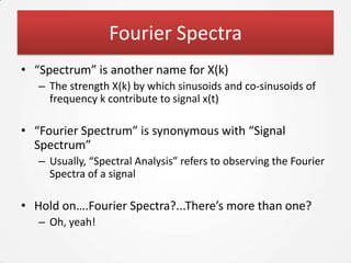
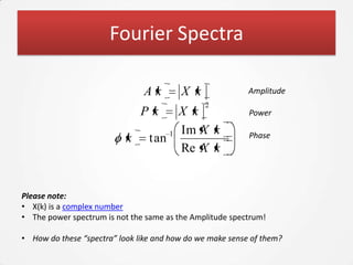
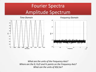
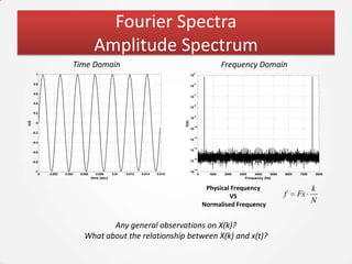
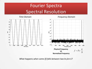
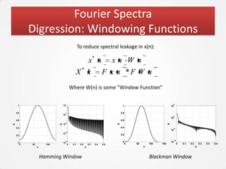
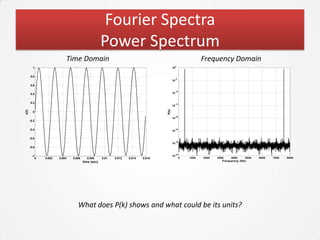
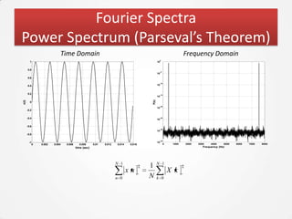
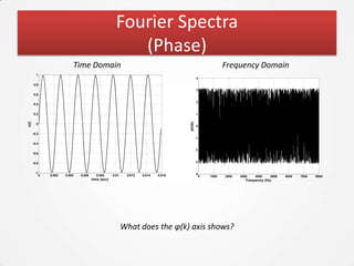
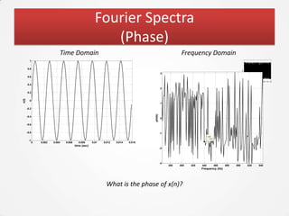
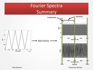
The document discusses the Fourier Transform and its application in signal processing, including the transformation of signals between time and frequency domains. It covers the basics of Fourier spectra, properties of the Fourier Transform, and practical applications in MATLAB for analyzing and visualizing signals. Additionally, it explores key concepts such as discrete Fourier Transform, spectral analysis, and the significance of phase in signal representation.


![Ch2 rev[1]](https://cdn.slidesharecdn.com/ss_thumbnails/ch2rev1-111122190305-phpapp01-thumbnail.jpg?width=640&height=640&fit=bounds)


