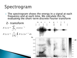
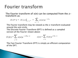
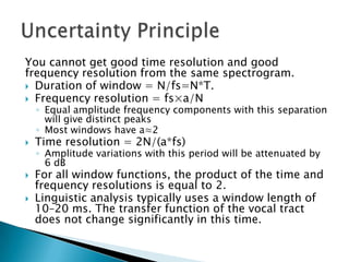
This lecture discusses spectrogram analysis and the short-term discrete Fourier transform. It defines normalized time and frequency, examines the effect of window length on time-frequency resolution, and derives descriptions of frequency and time resolution. It also reviews properties of the discrete Fourier transform and illustrates the uncertainty principle with examples.

1. Methods and algorithms of speech recognition
course
Nikolay V. Karpov
nkarpov(а)hse.ru
Lection 2

2.  This lecture is concerned with the spectrogram as a
representation of how the frequency components within a
signal vary with time.
 Define what we mean by normalised time and frequency
 Define the short-term discrete Fourier transformaton
 Look at the effect of different window lengths on time and
frequency resolution
 Derive a quantitative description of the frequency
resolution of the short term DFT and compare the
performance of common windows
 Derive a quantitative description of the time resolution of
the short term DFT
 Explain the uncertainty principle and illustrate its effects
with some examples
 Review some of the properties of the DFT

3. Sampling
theorem says
that when the
analog signal
x(t) is band-
restricted
between 0 and
W[Hz] and when
x(t) is sampled
at every T =
1/2W, the
original signal
can be
completely
reproduced by

4. For those signals the
frequency bandwidths of
which are not known, a
low-pass filter is used to
restrict the bandwidths
before sampling. When a
signal is sampled
contrary to the sampling
theorem, aliasing
distortion occurs, which
distorts the high-
frequency components of
the signal, as shown

5. Designate
sin(2 wt )
g (t )
2 wt
i i i i
x(t ) x( ) g (t ) x( ) x( ) x(iT ) x(i )
i 1 2w 2w 2w Fs
Simple continuous signal x(t )
A cos(2 ft )
i k
x(t ) A cos(2 f ( ) ) A cos( i ) A cos(2 i )
Fs N
1 k
Normalised radian frequency 0 2 f( ) 2 (1) 0.5
Fs N
Normalised time i

6. With sampled data systems it is customary to change
the time scale and work in units of the sample period.
 In normalised units the sampling frequency (fs) and
period (T) both equal 1. They can therefore be
omitted from equations: any such omissions can be
deduced using dimensional consistency arguments.
 The Nyquist frequency is ½ Hz = πradians/second
 To convert back to real units:
◦ any time quantity must be multiplied by the real sample
period (or divided by the real sample frequency)
◦ any frequency or angular frequency quantity must be
multiplied by the real sample frequency (or divided by the
real sample period)

7.  The spectrogram shows the energy in a signal at each
frequency and at each time. We calculate this by
evaluating the short-term discrete Fourier transform
Z- tramsform
n
X ( z) x ( n) z
n
1
X ( z) X ( z ) z n 1dz
2 j c

8. The Fourier transform of x(n) can be computed from the z-
transform as:
i n
X( ) X ( z) z e i x ( n )e
n
The Fourier transform may be viewed as the z-transform evaluated
around the unit circle.
The Discrete Fourier Transform (DFT) is defined as a sampled
version of the Fourier shown above:
N 1 N 1
i 2 kn / N
X (k ) x ( n )e x ( n) X ( k )e i 2 kn / N
n 0 n 0
The Fast Fourier Transform (FFT) is simply an efficient computation
of the DFT.

9.  The Discrete Cosine Transform (DCT) is simply a
DFT of a signal that is assumed to be real and
even (real and even signals have real spectra!)
N 1
X (k ) x(0) 2 x(n) cos(2 kn / N ); k 0,1,..., N 1
n 0
Note that these are not the only transforms used in
speech processing
 Wavelets;
 Fractals;
 Wigner distributions;
 etc.

10.  We often want to estimate the “power
spectrum” of a non-stationary signal at a
particular instant of time.
 Multiply by a finite length window and take
the DFT.
 For a window of length N ending on sample m
we have:
N 1
i 2 k (m n) / N
X ( k ; m) w(n) x(m n)e
n 0
k-frequency, m-time

11. 2
 X (k , m) X (k , m) X * (k , m) gives the power at a frequency of
k/N Hz (normalized) for a window centred at m-0.5(N-1).
 the (m-i) term in the exponent means that the phase origin
remains consistent by cancelling out the linear phase shift
introduced by a delay of m samples.
 the window samples are numbered backwards in time (for
convenience later) hence the summation is performed backwards
in time.
 The values X(k;m) are based on the N signal values from m–N+1
to m.
 the frequency resolution is 1/N Hz (normalised units)
 the spectrum is periodic and (since w and x are real) conjugate
symmetric:
X (k ) X (N k) X *( k)
 there are only 0.5N+1independent frequency values

12. Sound «is»
Hamming window of length
401 samples centred on 400

13. Line spectrum from larynx oscillation (at about 0.01
normalised Hz) is superimposed on vocal tract resonances

14.  Wide window (N=400)
 Independent frequency
values=N/2+1=201
 Short window eliminates the fine
detail (N=30)
 N/2+1=16
 Zero padded window gives more
spectrum points and an illusion of
more detail (N=480=30×16). This is
the normal case for a spectrogram
 N/2+1=241

15. N 1
X ( k ; m) w(n) x(m n) exp i 2 k ( m n) / N
n 0
By setting r= N–1–i we can rewrite this as:
2 j (m N 1) N 1
X ( k ; m) exp( ) * ym (r ) exp 2 jkr / N
N r 0
ym (r ) w( N 1 r ) x(m N 1 r )
This is a standard DFT multiplied by a phase-shift term that
is proportional to k: this compensates for the starting time
of the window: m–N+1
y(r) is a product of two signals so its DFT is the convolution
of the DFT’s of w(N–1–r) and x(m–N+1+r)

17. Rectangle window
w(n) 1
Slidelobe -13.3 dB
Mainlobe width(-3dB) 0.027
Leakage factor 9.14%
a=1.21, b=2
N
ck cos(2k (n ) / N)
2
Hamming window
w(n) 0.54 046 c1
Slidelobe -42.5 dB
Mainlobe width 0.039
Linkage factor 0.03%
a=1.81, b=4

18. Bartlett(L)
Blackman(L)
Rectwin(L)
Chebwin(L,R)
Hamming(L)
Hann(L)
Kaiser(L,beta)
taylorwin(L)
triang(L)

19. Спектр сигнала при использовании окна Блэкмана Спектр сигнала при использовании окна Блэкмана -
Наттала

20. BW = 45 Hz
NT = 44 ms
BW = 300 Hz
NT = 7 ms

21. /aI/ from “my” with 45Hz and 300Hz bandwidth spectrograms
45Hz, 44ms 300Hz, 7ms

22.  Vertical slice through
spectrogram:
 mT= 0.1s.
45 Hz gives finer frequency
resolution
 Horizontal slice through
spectrogram:
 k/NT= 3.5 kHz
300 Hz gives finer time
resolution

23. You cannot get good time resolution and good
frequency resolution from the same spectrogram.
 Duration of window = N/fs=N*T.
 Frequency resolution = fs×a/N
◦ Equal amplitude frequency components with this separation
will give distinct peaks
◦ Most windows have a≈2
 Time resolution = 2N/(a*fs)
◦ Amplitude variations with this period will be attenuated by
6 dB
 For all window functions, the product of the time and
frequency resolutions is equal to 2.
 Linguistic analysis typically uses a window length of
10–20 ms. The transfer function of the vocal tract
does not change significantly in this time.

24.  To keep all the information about time variation
of spectral components, you need only sample
the spectrum twice as fast as the spectral
magnitudes are varying. Using normalised
frequencies:
 –∞ dB bandwidth for an N-point window = b/N
◦ b = 4 for a Hamming window
 Significant variation of spectral components
occurs at frequencies below 2b/N
 we must sample the spectrum at a frequency of
b/N
◦ the separation between spectral samples is the window
width divided by b

25.  Exact line-spectrum of a periodic signal {xm}
 Sampled continuous spectrum of zero-extended {xm}
 Sampled continuous spectrum of infinite {xm} convolved with spectrum of
rectangular window
 FFT is an algorithm for calculating DFT
 Energy Conservation (Parseval’s theorem)
 Symmetries {xm} ⇒ {Xk}
 Discrete⇒Periodic:Xk+N=Xk
 Real⇒Hermitian: X–k= X*k
 Periodic:xm+N/r = x
 m ⇒Discrete:Xk= 0for k ≠ir
 Skew Periodic:xm+N/2r = –xm ⇒Odd Harmonics:
 Even:xm= x N–m ⇒Real
 Odd:xm= –x N–m ⇒Purely Imaginary
 Real & Even⇒Real & Even
 Real & Odd⇒Purely Imaginary and Odd