PPT on Discrete Fourier Transform ,Fast Fourier Transform and Windowing Techniques in detail step by step.Easy to learn and understand.

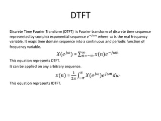
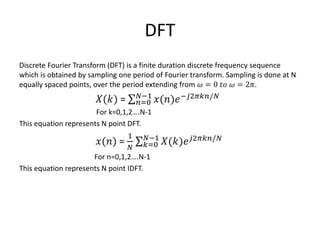
1. Presented By:
Abhishek Verma

2. DTFT
Discrete Time Fourier Transform (DTFT) is Fourier transform of discrete time sequence
represented by complex exponential sequence 𝑒−𝑗𝜔𝑛
where 𝜔 is the real frequency
variable. It maps time domain sequence into a continuous and periodic function of
frequency variable.
𝑋(𝑒 𝑗𝜔) = 𝑛=−∞
∞ 𝑥(𝑛)𝑒−𝑗𝜔𝑛
This equation represents DTFT.
It can be applied on any arbitrary sequence.
𝑥(𝑛) =
1
2𝜋 −𝜋
𝜋
𝑋(𝑒 𝑗𝜔)𝑒 𝑗𝜔𝑛 𝑑𝜔
This equation represents IDTFT.

3. DFT
Discrete Fourier Transform (DFT) is a finite duration discrete frequency sequence
which is obtained by sampling one period of Fourier transform. Sampling is done at N
equally spaced points, over the period extending from 𝜔 = 0 𝑡𝑜 𝜔 = 2𝜋.
𝑋(𝑘) = 𝑛=0
𝑁−1
𝑥(𝑛)𝑒−𝑗2𝜋𝑘𝑛/𝑁
For k=0,1,2….N-1
This equation represents N point DFT.
𝑥(𝑛) =
1
𝑁 𝑘=0
𝑁−1
𝑋(𝑘)𝑒 𝑗2𝜋𝑘𝑛/𝑁
For n=0,1,2….N-1
This equation represents N point IDFT.

4. Twiddle Factor
𝑊𝑁 = 𝑒−𝑗2𝜋/𝑁
This is called twiddle factor. It makes computation of DFT a bit easy and fast.
𝑋(𝑘) = 𝑛=0
𝑁−1
𝑥 𝑛 𝑊𝑁
𝑘𝑛
For k=0,1,2….N-1
This equation represents N point DFT.
𝑥(𝑛) =
1
𝑁 𝑘=0
𝑁−1
𝑋(𝑘)𝑊𝑁
−𝑘𝑛
For n=0,1,2….N-1
This equation represents N point IDFT.

5. DFT Properties
1. Periodicity
𝑥 𝑛 = 𝑥 𝑛 + 𝑁
𝑋 𝑘 = 𝑋[𝑘 + 𝑁]
2. Linearity
𝑎1 𝑥1 𝑛 + 𝑎2 𝑥2 𝑛
𝑎1 𝑋1 𝑘 + 𝑎2 𝑋2 𝑘
3. Time Reversal
𝑥[𝑁 − 𝑛]
𝑋[𝑁 − 𝑘]
4. Circular time shift
𝑥[𝑛 − 𝑙] 𝑁
X[𝑘]𝑒−𝑗2𝜋𝑘𝑙/𝑁

6. DFT Properties
5. Circular frequency shift
𝑥[𝑛]𝑒 𝑗2𝜋𝑙𝑛/𝑁
𝑋[𝑘 − 𝑙] 𝑁
6. Circular convolution
𝑥1[𝑛] ⊙ 𝑥2[𝑛]
𝑋1 𝑘 𝑋2[𝑘]
7. Circular correlation
𝑥 𝑛 ⊙ 𝑦⋇
−𝑛
𝑋 𝑘 𝑌⋇[𝑘]
8. Multiplication
𝑥1[𝑛]𝑥2 [𝑛]
1
𝑁
𝑋1[𝑘] ⊙ 𝑋2[𝑘]

7. DFT Properties
9. Complex conjugate
𝑥⋇[𝑛]
𝑋∗
[𝑁 − 𝑘]
10. Parseval’s Theorem
𝑛=0
𝑁−1
𝑥 𝑛 𝑦⋇ 𝑛
1
𝑁
𝑛=0
𝑁−1
𝑋 𝑘 𝑌⋇ 𝑘

8. Computational Complexity in DFT
In direct computation,
𝑋(𝑘) = 𝑛=0
𝑁−1
𝑥 𝑛 𝑊𝑁
𝑘𝑛
For k=0,1,2….N-1
We have
Complex multiplications
𝑁 ∗ 𝑁 = 𝑁2
Complex additions
𝑁 𝑁 − 1 = 𝑁2
− 𝑁

9. FFT
Fast Fourier Transform is used to reduce number of arithmetic operations involved in
the computation of DFT by using:
1. Radix-2 Decimation in Time(DIT) algorithm
2. Radix-2 Decimation in Frequency(DIF) algorithm
It uses following properties of twiddle factor:
1. Periodic
𝑊𝑁
𝑘+𝑁
= 𝑊𝑁
𝑘
2. Symmetric
𝑊𝑁
𝑘+
𝑁
2 = −𝑊𝑁
𝑘

10. Radix-2 DIT algorithm

11. Radix-2 DIF algorithm

12. Computational Complexity in FFT
𝑋 𝑚+1[𝑝] = 𝑋 𝑚[𝑝] + 𝑊𝑁
𝑟
𝑋 𝑚[𝑞]
𝑋 𝑚+1[𝑞] = 𝑋 𝑚 𝑝 − 𝑊𝑁
𝑟
𝑋 𝑚[𝑞]
We have
Complex multiplications
𝑁
2
log2 𝑁
Complex additions
𝑁 log2 𝑁

13. Resolution in FFT
When using FFT analysis to study the frequency
spectrum of signals, there are limits on resolution
between different frequencies, and on detectability
of a small signal in the presence of a large one.
There are two basic problems:
1. The fact that we can only measure the signal for
a limited time
2. The fact that the FFT only calculates results for
certain discrete frequency values (the 'FFT bins').

14. The sampled time waveform input to an FFT determines the computed spectrum. If an
arbitrary signal is sampled at a rate equal to 𝑓𝑠 over an acquisition time T, N samples are
acquired. Then Resolution Frequency is given by:
1
𝑇
=
𝑓𝑠
𝑁
Maximum Resolvable Frequency 𝑓𝑚𝑎𝑥
𝑓𝑚𝑎𝑥 =
𝑓𝑠
2
Minimum Resolvable Frequency 𝑓 𝑚𝑖𝑛
𝑓 𝑚𝑖𝑛= 0
The following strategies achieve a finer frequency resolution:
1. Decrease the sampling frequency, fs. Decreasing fs usually is not practical because
decreasing fs reduces the frequency range.
2. Increase the number of samples, N. Increasing N yields an increased number of lines
over the original frequency range.

15. Analyze a signal that contains two tones at 1,000 Hz and 1,100 Hz, use a sampling
frequency of 10,000 Hz. Acquire data for 10 ms with a frequency resolution of 100 Hz.
The following front panel shows the results of this analysis.

16. Increase the acquisition time to 1 s to achieve a frequency resolution of 1 Hz. The
following front panel shows the results obtained with a 1 s acquisition time.

17. Rectangular Window
The rectangular window takes all samples with equal weight into account. The main
lobe of its magnitude spectrum is narrow, but the level of the side lobes is rather
high. It has the highest frequency selectivity.
𝑊𝑅 𝑛 =
1 , 0 < 𝑛 < 𝑀 − 1
0 , 𝑒𝑙𝑠𝑒𝑤ℎ𝑒𝑟𝑒

18. Triangular Window
For an odd window length 2N−1 , the triangular window can be expressed as the
convolution of two rectangular windows. The main lobe is wider as for the
rectangular window, but the level of the side lobes decays faster.
𝑊𝑇 𝑛 = 1 −
2 𝑛
𝑀 − 1
, 𝑛 ≤ 𝑀 − 1

19. Hanning Window
The Hanning window is a smooth window whose first and last value is zero. It features
a fast decay of the side lobes.
𝑊ℎ𝑛 𝑛 =
1
2
1 − cos
2𝜋𝑛
𝑀 − 1

20. Hamming Window
The Hamming window is a smooth window function whose first and last value is not
zero. The level of the side lobes is approximately constant.
𝑊ℎ𝑚 𝑛 = 0.54 + 0.46 cos
2𝜋𝑛
𝑀 − 1
0 , 𝑒𝑙𝑠𝑒𝑤ℎ𝑒𝑟𝑒

21. Blackman Window
The Blackman window features a rapid decay of side lobes at the cost of a wide main
lobe and low frequency selectivity.
𝑊𝐵 𝑛 = 0.42 + 0.5 cos
2𝜋𝑛
𝑀 − 1
+ 0.08 cos
4𝜋𝑛
𝑀 − 1

22. Applications
1. It can be used in spectral analysis.
2. It can be used in signal processing.
3. It can be used in image processing.