Download as PDF, PPTX
![Ideal Sampling
3/11/2019 3
Dr Naim R Kidwai, Professor, Integral University, Lucknow
www.nrkidwai.wordpress.com
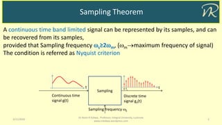
Let continuous time band limited signal be
0)(..)()( m
GtsGtg
Let periodic impulse train be
)(
1
)(or
])([*)(
2
1
)]([)(
)()()(signalSampledThen
2where;)()()(
n
s
s
n
ss
p
s
s
n
ss
k
sp
nG
T
G
nGtgFG
ttgtg
T
nTtt
Discrete time signal g(t)
Ideal
SamplingContinuous time signal g(t)
Sampling
frequency S
t tTs0
p(t)
tTs0
1
Using linearity property of FT and convolution property of impulse
n
s
s
nG
T
tg )(
1
)(Thus
Using multiplication property of FT](https://image.slidesharecdn.com/sampling-190311053856/85/Sampling-Theorem-3-320.jpg)
![Ideal Sampling
3/11/2019 4
Dr Naim R Kidwai, Professor, Integral University, Lucknow
www.nrkidwai.wordpress.com
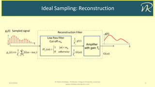
g(t) Signal
t
g(t) Sampled signal
tTs 2Ts0 3Ts
p(t) Impulse train
tTs 2Ts0 3Ts
1
p()
s 2s0
s
-s-2s
G()
m-m
A
F[g(t)]
s 2s0
A/Ts
-s-2s
s> 2m
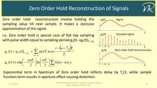
In Time domain:
Sampling results in conversion of
continuous time signal into discrete time
signal
In Frequency domain:
Sampling results in multiple translation of
signal spectrum (linear combination of
shifted signal spectrum at integer
multiples of sampling frequency.](https://image.slidesharecdn.com/sampling-190311053856/85/Sampling-Theorem-4-320.jpg)
![Aliasing
3/11/2019 7
Dr Naim R Kidwai, Professor, Integral University, Lucknow
www.nrkidwai.wordpress.com
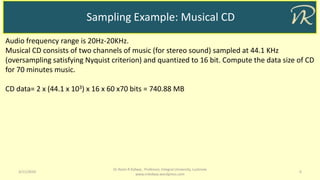
g(t) Signal
t
g(t) Sampled signal
tTs 2Ts0 3Ts
G()
m-m
A
F[g(t)]
s 2s0
As
-s-2s
s> 2m
In case of under sampling (s<2m),
shifted versions of signal spectrum shall
overlap resulting in spectral distortions.
In such case, signal can not be recovered
from its samples. This effect is known as
ALIASING.
To avoid aliasing effect due to spurious
frequencies, a pre alias filter is applied
before sampling
F[g(t)]
s 2s0
As
-s-2s
s= 2m
s <2m
F[g(t)]
s 2s0
As
-s-2s
g(t) Sampled signal
tTs 2Ts0 3Ts
g(t) Sampled signal
tTs 2Ts0 3Ts
](https://image.slidesharecdn.com/sampling-190311053856/85/Sampling-Theorem-7-320.jpg)

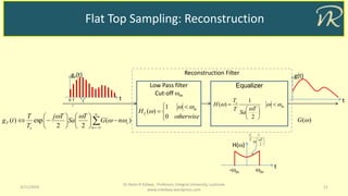
![Flat Top Sampling
3/11/2019 10
Dr Naim R Kidwai, Professor, Integral University, Lucknow
www.nrkidwai.wordpress.com
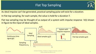
g(t) Signal
t
g(t) Sampled signal
tTs 2Ts0 3Ts
p(t) Impulse train
tTs 2Ts0 3Ts
1
p()
s 2s0
s
-s-2s
G()
m-m
A
F[g(t)]
s 2s0
As
-s-2s
s> 2m
F[gF(t)]
s 2s0
As
-s-2s
s> 2m
gF(t)
tTs0 T
Flat top sampling, introduces aperture effect as per sample function](https://image.slidesharecdn.com/sampling-190311053856/85/Sampling-Theorem-10-320.jpg)
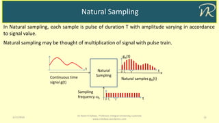
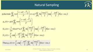
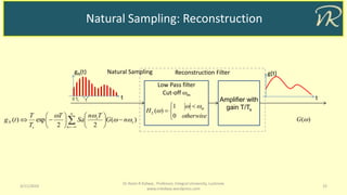
![Natural Sampling
3/11/2019 14
Dr Naim R Kidwai, Professor, Integral University, Lucknow
www.nrkidwai.wordpress.com
g(t) Signal
t
s 2s0
sT
-s-2s
G()
m-m
A
F[gN(t)]
s 2s0
As
-s-2s
s> 2m
tTs0 T
Pulse Train
Natural sampling, introduces amplitude scaling as per sample function at every shifted version
of G(), and not the aperture effect as in Flat top sampling.
gN(t) Natural Sampling
tTs0 T](https://image.slidesharecdn.com/sampling-190311053856/85/Sampling-Theorem-14-320.jpg)
![Discrete Time Processing of Continuous time Signals
3/11/2019 19
Dr Naim R Kidwai, Professor, Integral University, Lucknow
www.nrkidwai.wordpress.com
Continuous time signals can be converted into discrete time using sampling and quantized to
make it digital. These discrete time signals can be processed using computer based discrete
time systems and output can be reconstructed as continuous time signal.
g(t) A/D converter
(Sampling/
Quantization)
Discrete time
system
D/A converter
(Reconstruction)
g(nTs)
=g[n]
y(nTs)
=y[n] y(t)](https://image.slidesharecdn.com/sampling-190311053856/85/Sampling-Theorem-19-320.jpg)

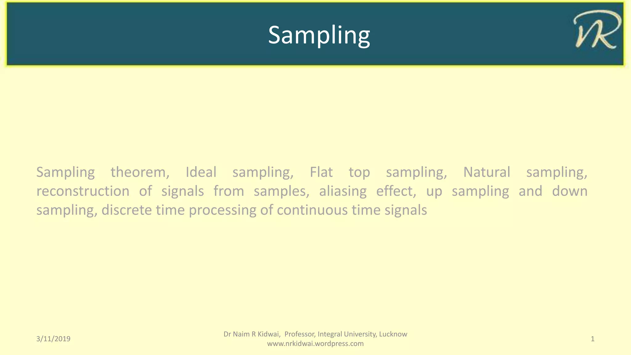
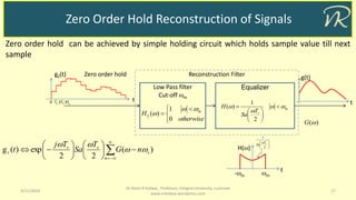
The document discusses various sampling methods for continuous signals, including ideal sampling, natural sampling, and flat top sampling, emphasizing the Nyquist criterion for accurate signal recovery. It explains the effects of aliasing in under-sampling and presents practical examples, such as the sampling process in audio CDs. Reconstruction techniques, such as zero order hold and the application of low pass filters, are also covered to illustrate how to recover the original signal from its samples.


![Digital Signal Processing[ECEG-3171]-Ch1_L05](https://cdn.slidesharecdn.com/ss_thumbnails/dspl5ch2-180427094424-thumbnail.jpg?width=640&height=640&fit=bounds)