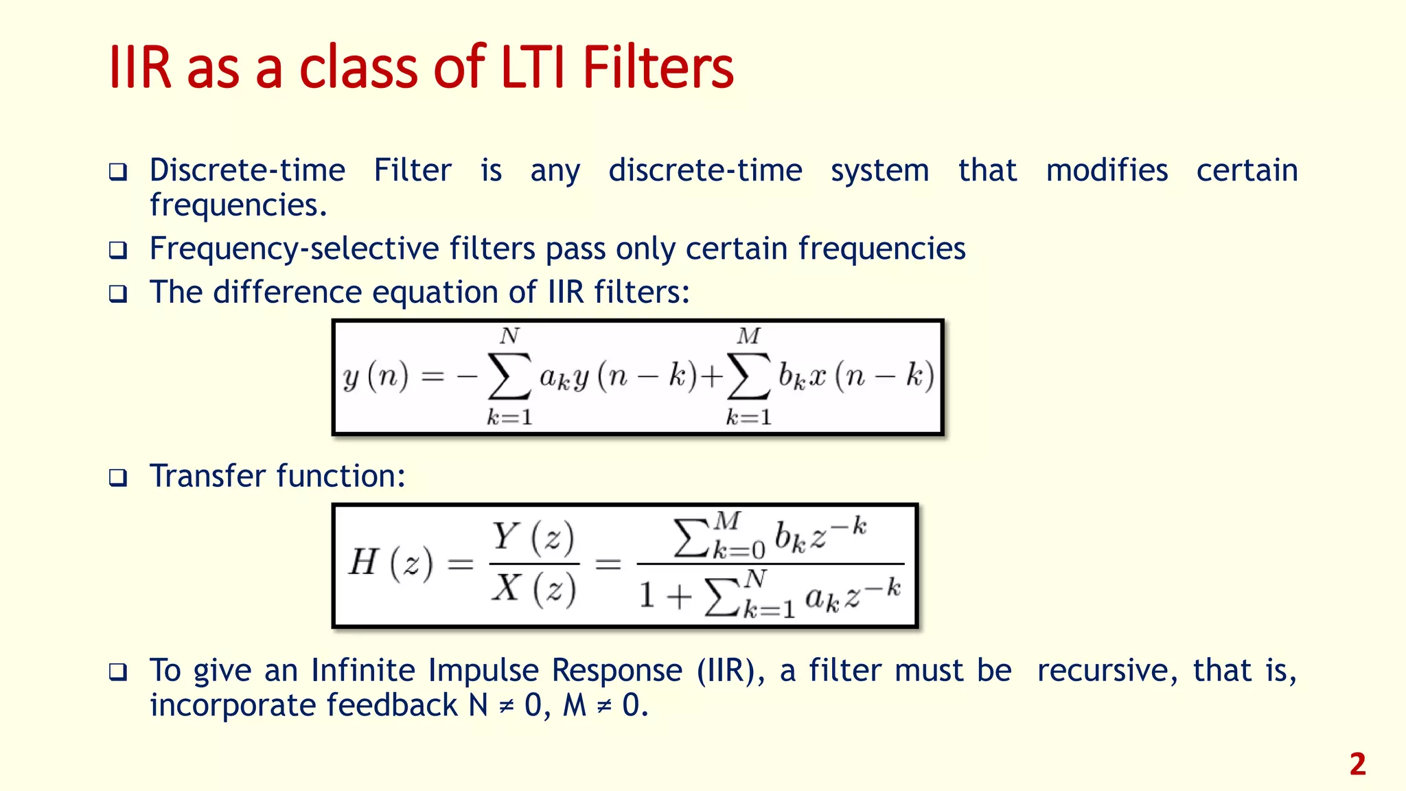
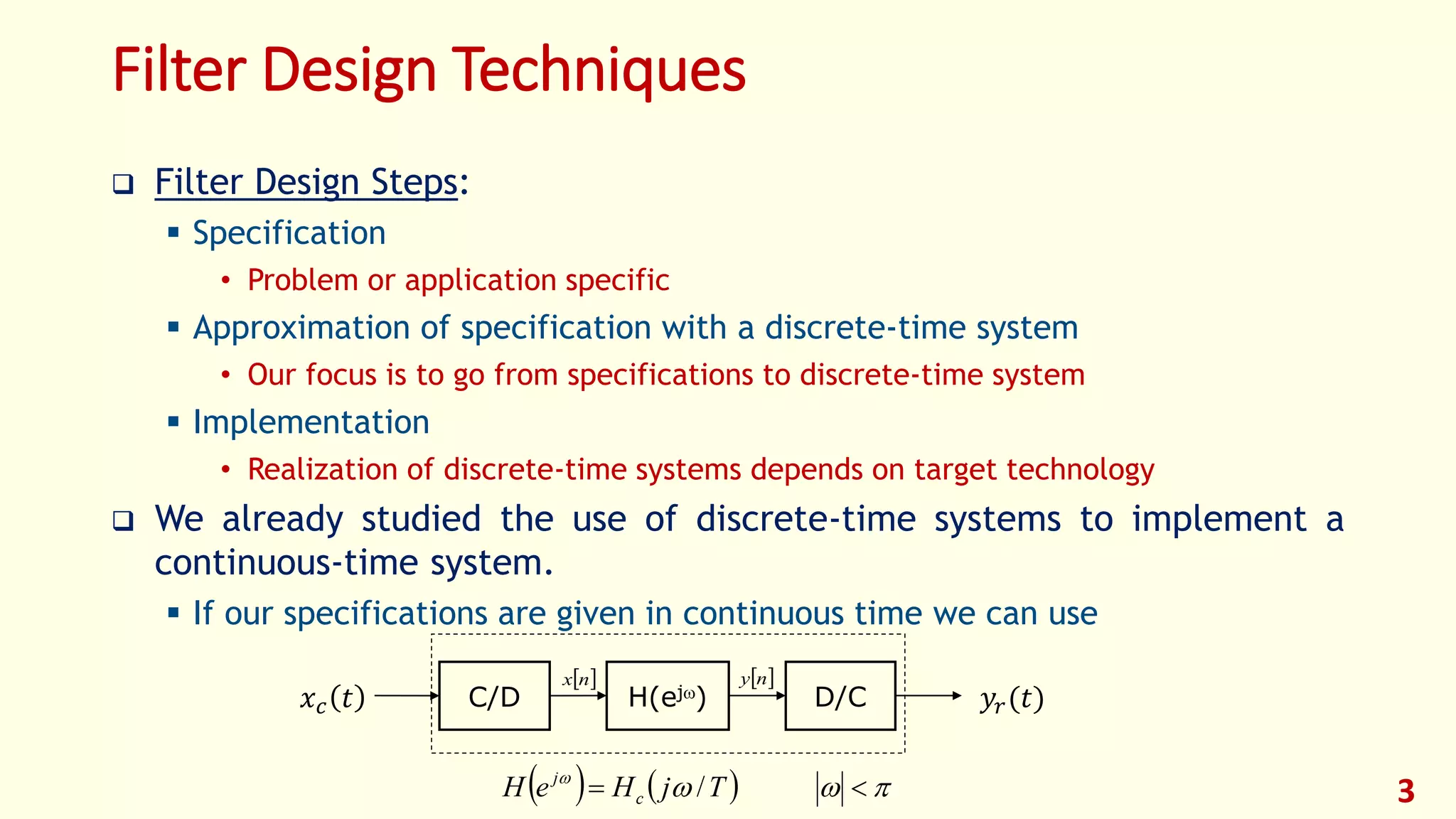
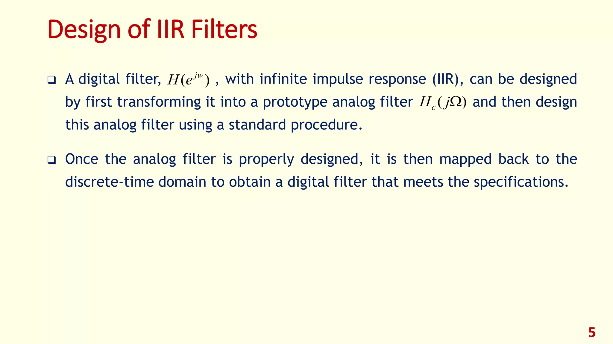
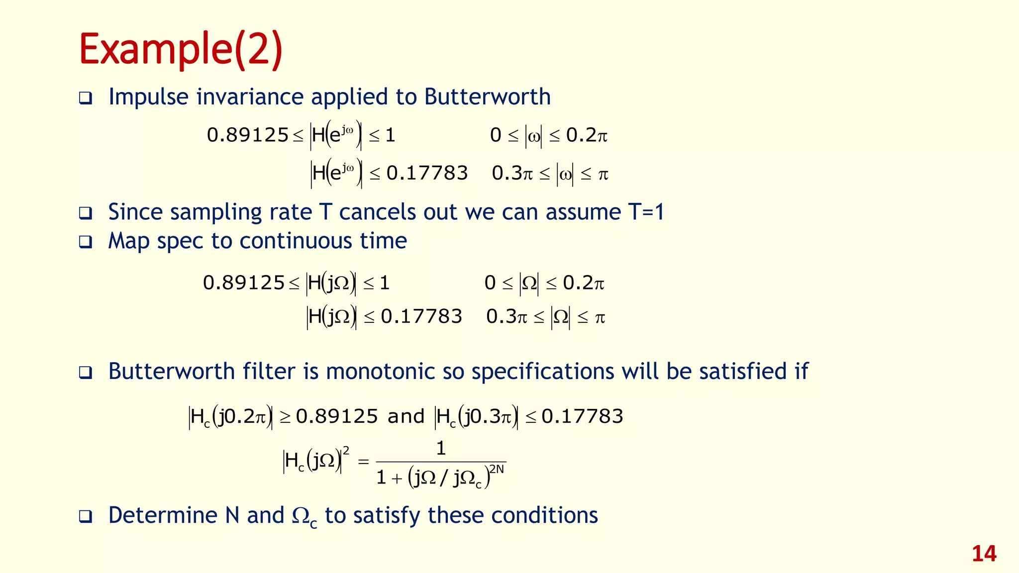
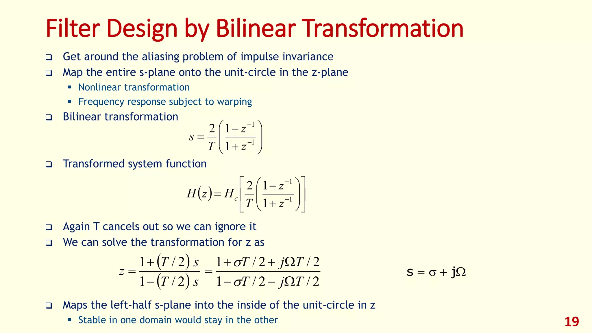
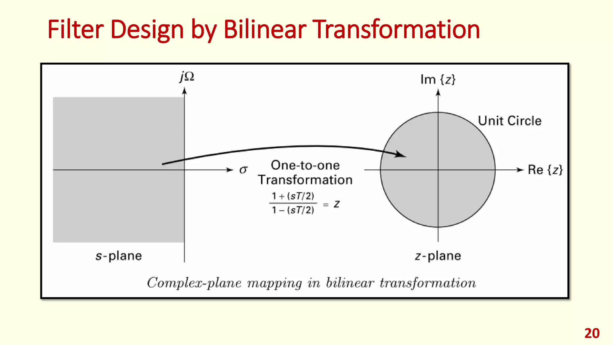
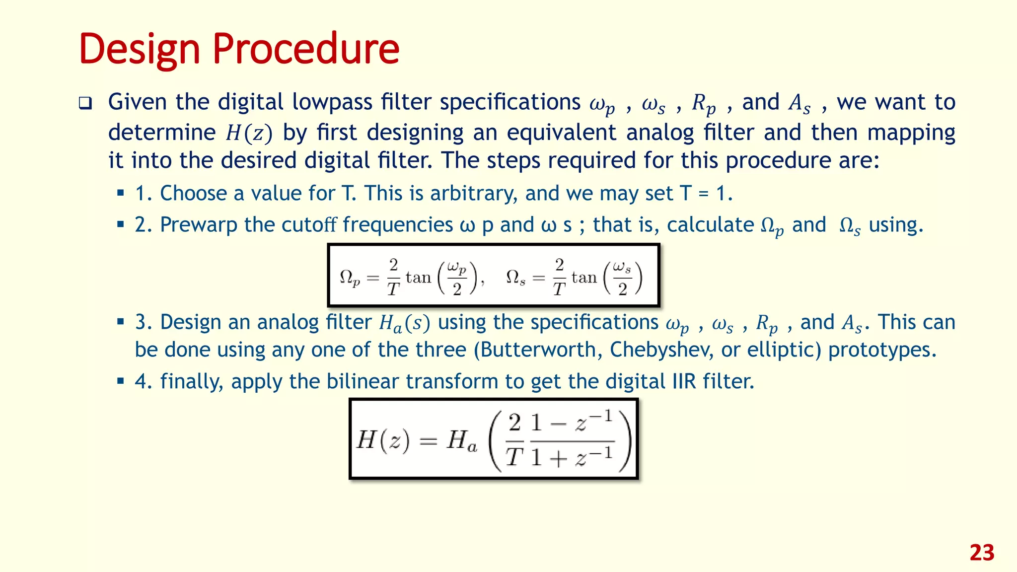
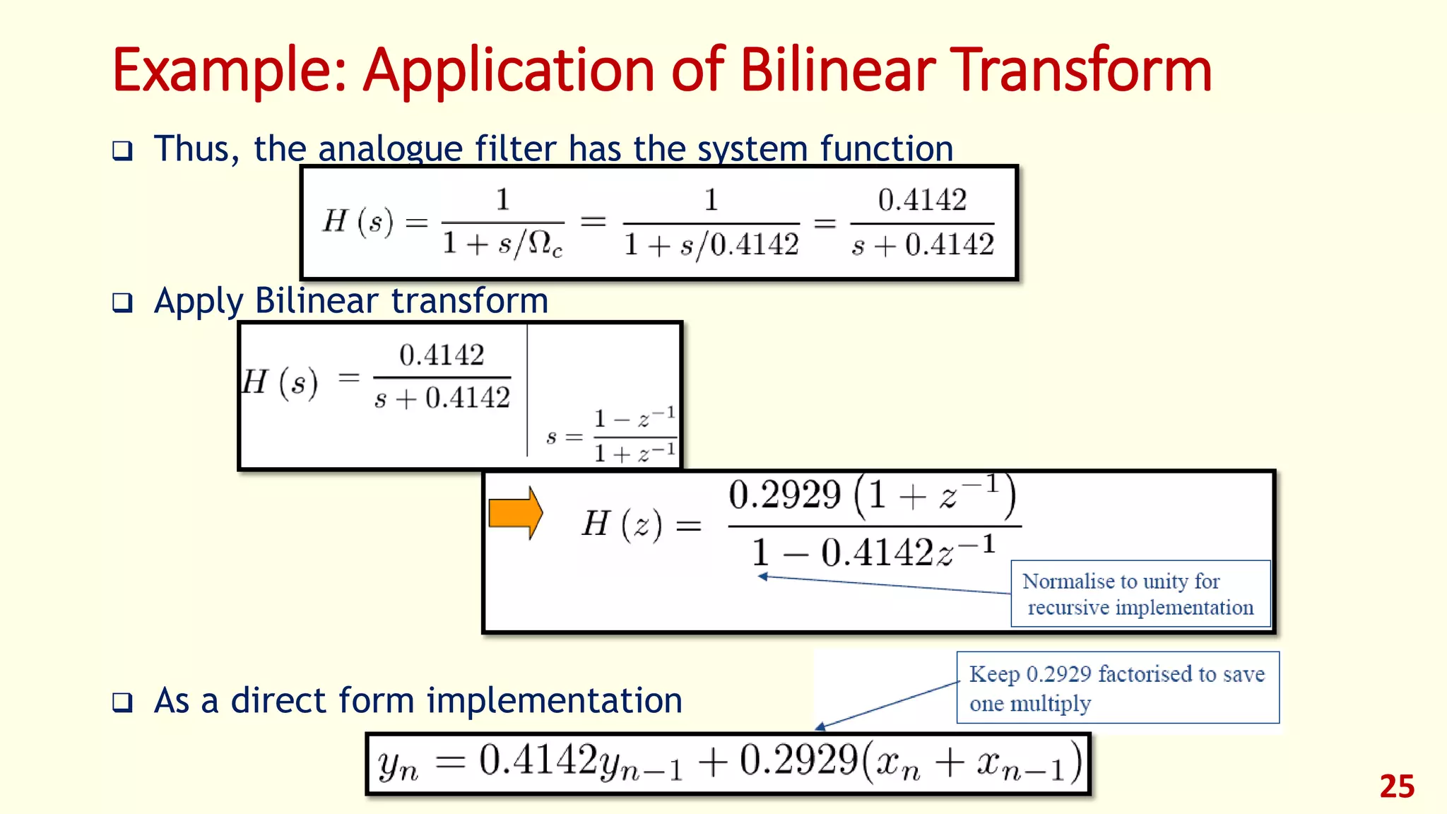
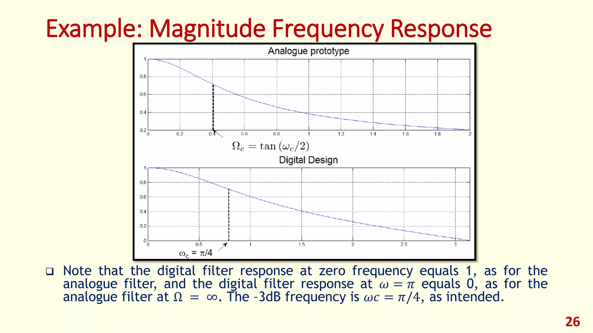
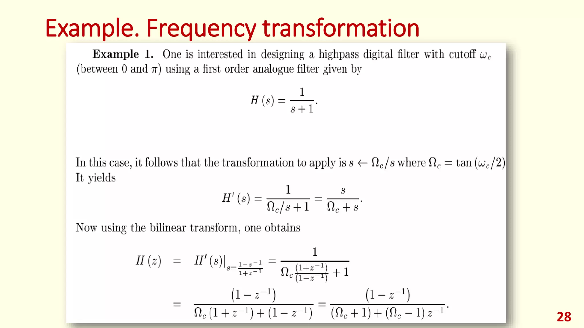
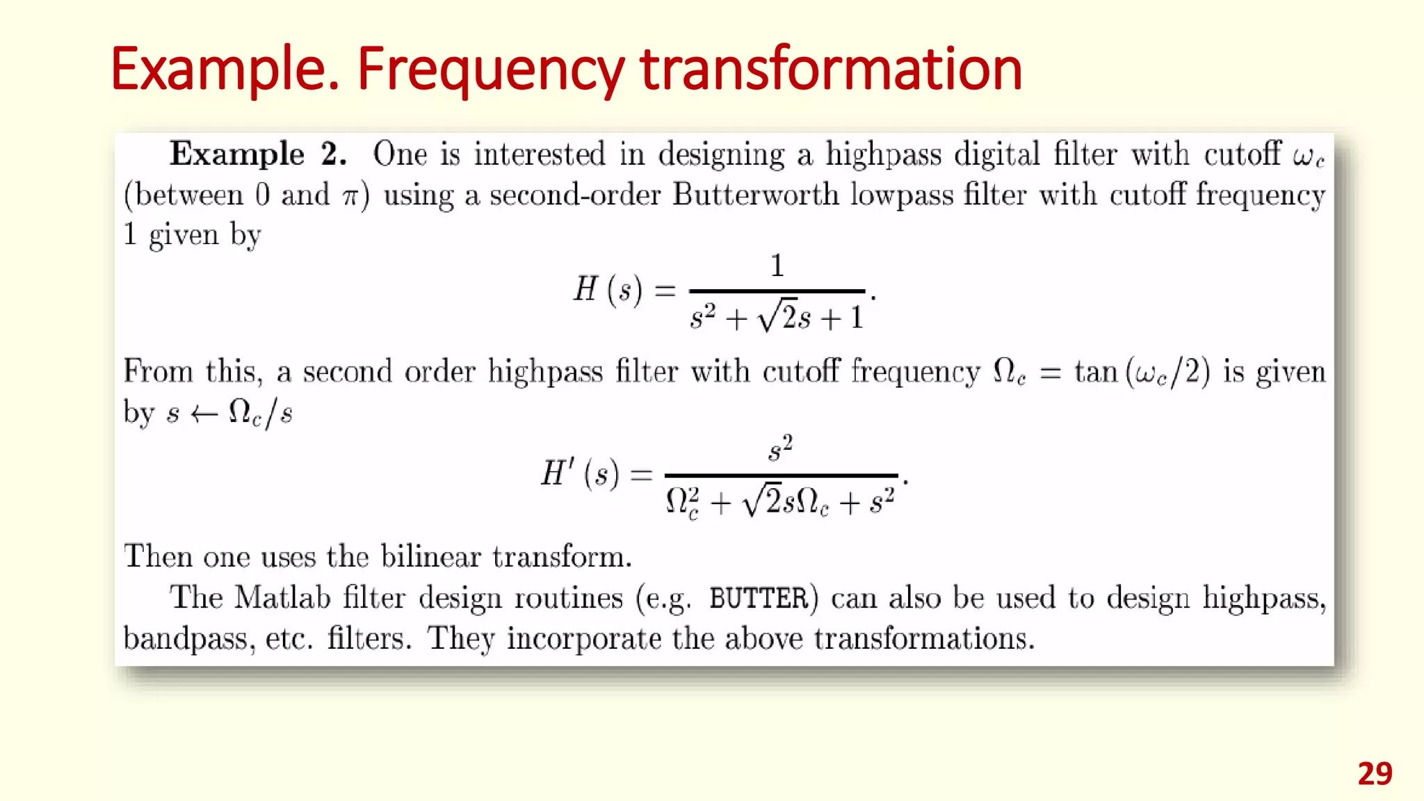
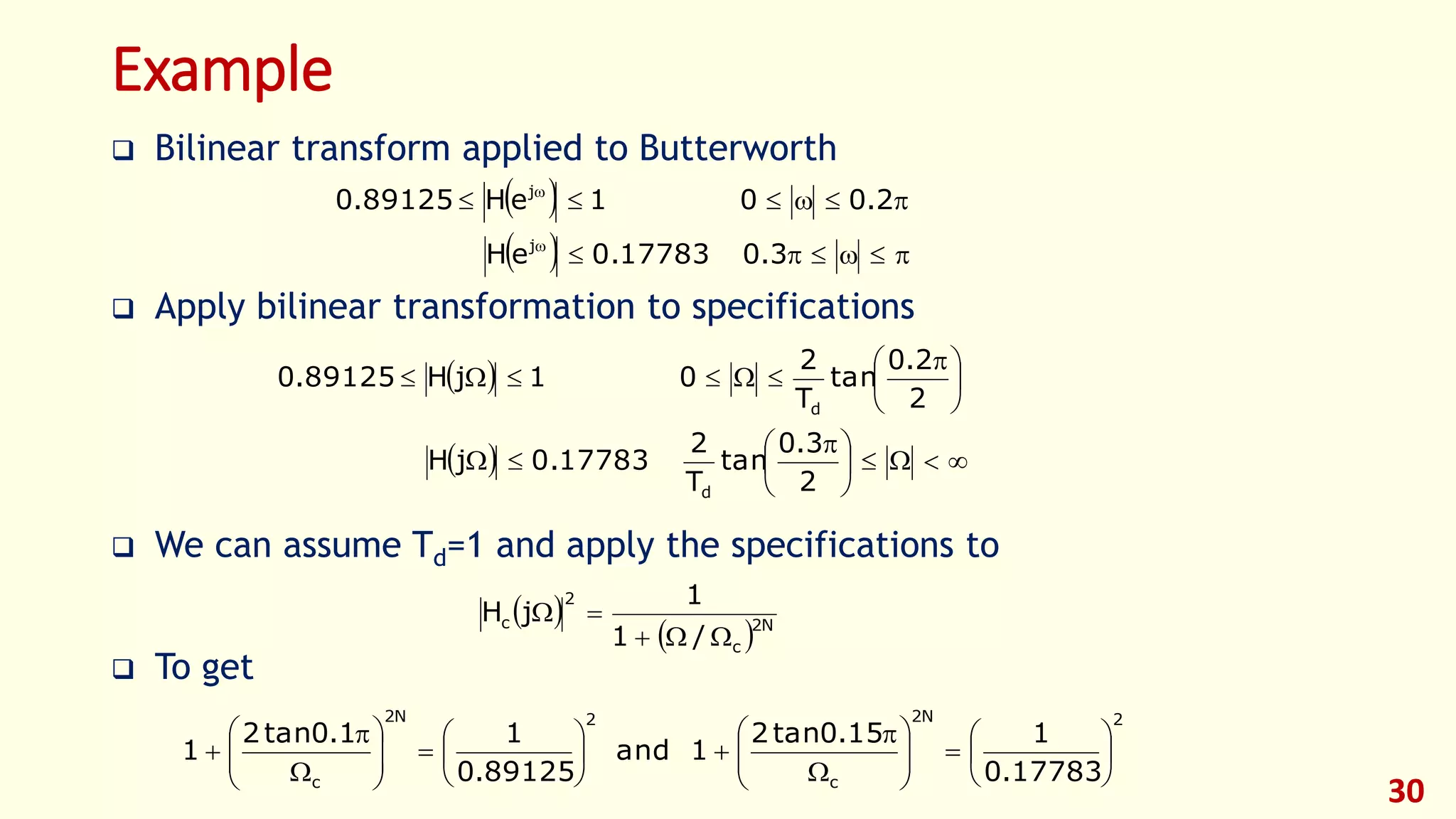
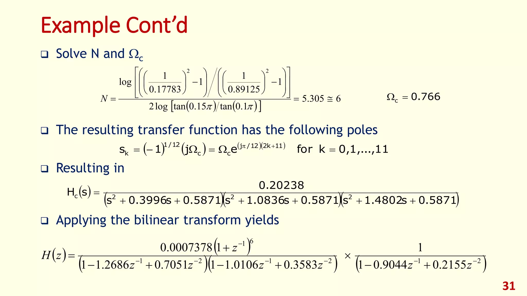
The document discusses techniques for designing discrete-time infinite impulse response (IIR) filters from continuous-time filter specifications. It covers the impulse invariance method, matched z-transform method, and bilinear transformation method. The impulse invariance method samples the continuous-time impulse response to obtain the discrete-time impulse response. The bilinear transformation maps the entire s-plane to the unit circle in the z-plane to avoid aliasing. Examples are provided to illustrate the design process using each method.

1. ‫ر‬َ‫ـد‬ْ‫ق‬‫ِـ‬‫ن‬،،،‫لما‬‫اننا‬ ‫نصدق‬ْْ‫ق‬ِ‫ن‬‫ر‬َ‫د‬
LECTURE (11)
Discrete-Time IIR Filter Design from
Continuous-Time Filters
Assist. Prof. Amr E. Mohamed

2. IIR as a class of LTI Filters
 Discrete-time Filter is any discrete-time system that modifies certain
frequencies.
 Frequency-selective filters pass only certain frequencies
 The difference equation of IIR filters:
 Transfer function:
 To give an Infinite Impulse Response (IIR), a filter must be recursive, that is,
incorporate feedback N ≠ 0, M ≠ 0.
2

3. 3
Filter Design Techniques
 Filter Design Steps:
 Specification
• Problem or application specific
 Approximation of specification with a discrete-time system
• Our focus is to go from specifications to discrete-time system
 Implementation
• Realization of discrete-time systems depends on target technology
 We already studied the use of discrete-time systems to implement a
continuous-time system.
 If our specifications are given in continuous time we can use
D/C𝑥 𝑐 𝑡 𝑦𝑟(𝑡)C/D H(ej)
 nx  ny
    
 /TjHeH c
j

4. Filter Specifications
 Specifications
 Passband
 Stopband
 Parameters
 Specifications in dB
 Ideal passband 𝑔𝑎𝑖𝑛 = 20log(1) = 0 𝑑𝐵
 Max passband 𝑔𝑎𝑖𝑛 = 20log(1.01) = 0.086𝑑𝐵
 Max stopband 𝑔𝑎𝑖𝑛 = 20log(0.001) = −60 𝑑𝐵
4
   20002001.199.0  forjHeff
     30002001.0 forjHeff
 
 30002
20002
001.0
01.0
2
1








s
p

5. Design of IIR Filters
 A digital filter, , with infinite impulse response (IIR), can be designed
by first transforming it into a prototype analog filter and then design
this analog filter using a standard procedure.
 Once the analog filter is properly designed, it is then mapped back to the
discrete-time domain to obtain a digital filter that meets the specifications.
5
)( jw
eH
)( jHc

6. Design of IIR Filters
 The commonly used analog filters are
1. Butterworth filters: no ripples at all,
2. Chebyshev filters: ripples in the passband OR in the stopband, and
3. Elliptical filters: ripples in BOTH the pass and stop bands.
 A disadvantage of IIR filters is that they usually have nonlinear phase.
Some minor signal distortion is a result.
 There are two main techniques used to design IIR filters:
1. The Impulse Invariant method,
2. Matched z-transform method, and
3. The Bilinear transformation method.
6

7. Butterworth Low Pass Filters
 Passband is designed to be maximally flat
 The magnitude square response of a Butterworth filter of order N is
 where is the 3-dB frequency of the filter.
 The larger N is, the closer the Butterworth filter is to an ideal low pass filter.
7
 
  N2
c
2
c
j/j1
1
jH

  
  N2
c
2
c
j/s1
1
sH


c

8. 8
Chebyshev Filters
 Equiripple in the pass-band and monotonic in the stop-band
 The magnitude square response of a N-th order Chebyshev filter with a
ripple parameter of ε is
 Where is the N-th order Chebyshev polynomial.
 
 
   xNxVwhere
V
jH N
cN
c
1
22
2
coscos
/1
1 




 xVN

9. 9
Filter Design by Impulse Invariance
 In this design method we want the digital filter impulse response to look “similar”
to that of a frequency-selective analog filter. Hence we sample ℎ 𝑎(𝑡) at some
sampling interval T to obtain h(n); that is,
 Mapping a continuous-time impulse response to discrete-time
 Mapping a continuous-time frequency response to discrete-time
 The analog and digital frequencies are related by 𝜔 = Ω𝑇 𝑜𝑟 𝑒 𝑗𝜔 = 𝑒 𝑗Ω𝑇 𝑜𝑟 𝑧 = 𝑒 𝑠𝑇
 If the continuous-time filter is band-limited to
   nThnh c
  









k
c
j
k
T
j
T
jH
T
eH
 21
  








1
d
c
j
T
jH
T
eH
  dc TjH /for0 

10. Design Procedure
 Given the digital lowpass filter specifications 𝜔 𝑝 , 𝜔𝑠 , 𝑅 𝑝 , and 𝐴 𝑠 , we want to
determine 𝐻(𝑧) by first designing an equivalent analog filter and then mapping
it into the desired digital filter. The steps required for this procedure are:
 1. Choose T and determine the analog frequencies
 2. Design an analog filter 𝐻 𝑎(𝑠) using the specifications 𝜔 𝑝 , 𝜔𝑠 , 𝑅 𝑝 , and 𝐴 𝑠. This can
be done using any one of the three (Butterworth, Chebyshev, or elliptic) prototypes.
 3. Using partial fraction expansion, expand 𝐻 𝑎(𝑠) into
 4. Now transform analog poles {𝑝 𝑘} into digital poles {𝑒 𝑝 𝑘 𝑇
} to obtain the digital
filter:
10

11. 11
Impulse Invariant method: Steps
 Sample the impulse response (quickly enough to avoid aliasing
problem)
 Compute z-transform of resulting sequence
 First order:
 Second Order:
aT
ez
z
zH
as
sH 



 )(
1
)(
aTaT
aT
ebTezz
bTezz
zH
bas
as
sH 22
2
22
)cos(2
)cos(
)(
)(
)(
)( 







aTaT
aT
ebTezz
bTez
zH
bas
b
sH 2222
)cos(2
)sin(
)(
)(
)( 






12. 12
Summary of the Impulse Invariant Method
 Advantage:
 preserves the order and stability of the analogue filter.
 The frequencies Ω and ω are linearly related.
 Disadvantages:
 There is distortion of the shape of frequency response due to aliasing.

13. Example(1)
 If the analog filter transfer function is
 Find the digital filter
 Combine the second and third terms, we obtain
13

14. 14
Example(2)
 Impulse invariance applied to Butterworth
 Since sampling rate T cancels out we can assume T=1
 Map spec to continuous time
 Butterworth filter is monotonic so specifications will be satisfied if
 Determine N and c to satisfy these conditions
 
  



3.00.17783eH
2.001eH89125.0
j
j
 
  

3.00.17783jH
2.001jH89125.0
    0.177833.0jHand89125.02.0jH cc 
 
  N2
c
2
c
j/j1
1
jH



15. 15
Example Cont’d
 Satisfy both constrains
 Solve these equations to get
 N must be an integer so we round it up to meet the spec
 Poles of transfer function
 The transfer function
 Mapping to z-domain
2N2
c
2N2
c 17783.0
13.0
1and
89125.0
12.0
1 




























70474.0and68858.5N c 
      
0,1,...,11kforej1s 11k212/j
cc
12/1
k  
  21
1
21
1
21
1
257.09972.01
6303.08557.1
3699.00691.11
1455.11428.2
6949.02971.11
4466.02871.0















zz
z
zz
z
zz
z
zH
 
   4945.0s3585.1s4945.0s9945.0s4945.0s364.0s
12093.0
sH 222



16. 16
Example Cont’d

17. Matched z-transform method
 Matched z-Transform: very simple method to convert analog filter into digital
filters.
 Poles and zeros are transformed according to
 Where Td is the sampling period
 Poles using this method are similar to impulse invariant method.
 Zeros are located at a new position.
 This method suffers from aliasing problem.
17

18. 18
Example of Impulse Invariant vs Matched z transform methods
 Consider the following analog filter into a digital IIR filter
 Impulse invariant method
 Matched z-transform
 Some poles but different zeros

19. 19
Filter Design by Bilinear Transformation
 Get around the aliasing problem of impulse invariance
 Map the entire s-plane onto the unit-circle in the z-plane
 Nonlinear transformation
 Frequency response subject to warping
 Bilinear transformation
 Transformed system function
 Again T cancels out so we can ignore it
 We can solve the transformation for z as
 Maps the left-half s-plane into the inside of the unit-circle in z
 Stable in one domain would stay in the other








 

1
1
1
12
z
z
T
s
  













 

1
1
1
12
z
z
T
HzH c
 
  2/2/1
2/2/1
2/1
2/1
TjT
TjT
sT
sT
z








 js

20. 20
Filter Design by Bilinear Transformation

21. 21
Bilinear Transformation
 On the unit circle the transform becomes
 To derive the relation between  and 
 Which yields




 j
d
d
e
2/Tj1
2/Tj1
z
 
 




















 



2
tan
2
2/cos2
2/sin22
1
12
2/
2/







T
j
e
je
T
j
e
e
T
s j
j
j
j
d





 







2
arctan2or
2
tan
2 T
T



22. 22
Bilinear
Transformation

23. Design Procedure
 Given the digital lowpass filter specifications 𝜔 𝑝 , 𝜔𝑠 , 𝑅 𝑝 , and 𝐴 𝑠 , we want to
determine 𝐻(𝑧) by first designing an equivalent analog filter and then mapping
it into the desired digital filter. The steps required for this procedure are:
 1. Choose a value for T. This is arbitrary, and we may set T = 1.
 2. Prewarp the cutoff frequencies ω p and ω s ; that is, calculate Ω 𝑝 and Ω 𝑠 using.
 3. Design an analog filter 𝐻 𝑎(𝑠) using the specifications 𝜔 𝑝 , 𝜔𝑠 , 𝑅 𝑝 , and 𝐴 𝑠. This can
be done using any one of the three (Butterworth, Chebyshev, or elliptic) prototypes.
 4. finally, apply the bilinear transform to get the digital IIR filter.
23

24. Example: Application of Bilinear Transform
 Design a first order low-pass digital filter with -3dB frequency of 1kHz
and a sampling frequency of 8kHz using a the first order analogue low-
pass filter
 which has a gain of 1 (0dB) at zero frequency, and a gain of -3dB ( =
√0.5 ) at Ωc rad/sec (the "cutoff frequency ").
 Solution:
 First calculate the normalized digital cutoff frequency:
 Calculate the equivalent pre-warped analogue filter cutoff frequency
(rad/sec)
24

25. Example: Application of Bilinear Transform
 Thus, the analogue filter has the system function
 Apply Bilinear transform
 As a direct form implementation
25

26. Example: Magnitude Frequency Response
 Note that the digital filter response at zero frequency equals 1, as for the
analogue filter, and the digital filter response at 𝜔 = 𝜋 equals 0, as for the
analogue filter at Ω = ∞. The –3dB frequency is 𝜔𝑐 = 𝜋/4, as intended.
26

27. Example: Pole-zero diagram for digital design
 Note that:
 The filter is stable, as expected
 The design process has added an extra zero compared to the prototype
• This is typical of filters designed by the bilinear transform.
27

28. Example. Frequency transformation
28

29. Example. Frequency transformation
29

30. 30
Example
 Bilinear transform applied to Butterworth
 Apply bilinear transformation to specifications
 We can assume Td=1 and apply the specifications to
 To get
 
  



3.00.17783eH
2.001eH89125.0
j
j
 
  




 






 

2
3.0
tan
T
2
0.17783jH
2
2.0
tan
T
2
01jH89125.0
d
d
 
  N2
c
2
c
/1
1
jH


2N2
c
2N2
c 17783.0
115.0tan2
1and
89125.0
11.0tan2
1 





























31. 31
Example Cont’d
 Solve N and c
 The resulting transfer function has the following poles
 Resulting in
 Applying the bilinear transform yields
    
6305.5
1.0tan15.0tanlog2
1
89125.0
1
1
17783.0
1
log
22







































N 766.0c 
      
0,1,...,11kforej1s 11k212/j
cc
12/1
k  
 
   5871.0s4802.1s5871.0s0836.1s5871.0s3996.0s
20238.0
sH 222c


   
    212121
61
2155.09044.01
1
3583.00106.117051.02686.11
10007378.0







zzzzzz
z
zH

32. 32
Example Cont’d

33. 33