This document discusses analysis of continuous time signals. It begins by introducing Fourier series representation of periodic signals using trigonometric and exponential forms. It describes properties of Fourier series such as linearity, time shifting, and frequency scaling. It then introduces the Fourier transform which transforms signals from the time domain to the frequency domain. Common Fourier transform pairs are listed. The Laplace transform is also introduced which transforms signals from the time domain to the complex s-domain. Key properties of the Laplace transform include linearity, scaling, time shifting, and the initial and final value theorems. Conditions for the existence of the Laplace transform are also provided.
Introduction to EC208 Signals and Systems course, covering continuous time signals and detailed contents of Fourier series, Fourier transform, and Laplace transform.
Signals represent physical quantities varying over time/space; Continuous Time Signals (CTS) vary continuously, while Discrete Time Signals (DTS) consist of discrete values.
Fourier series represents periodic signals using sine and cosine functions; highlights periodic signal conditions and derivation of Fourier coefficients.
Key properties of CT Fourier Series including linearity, time shifting, frequency shifting, scaling, and differentiation/integration capabilities.
Parseval's Theorem links time and frequency domains for energy signals; examines Trigonometric and Exponential Fourier Series and their orthogonality.
Fourier Transform expands Fourier series applicability for non-periodic signals; derivation process discussed.
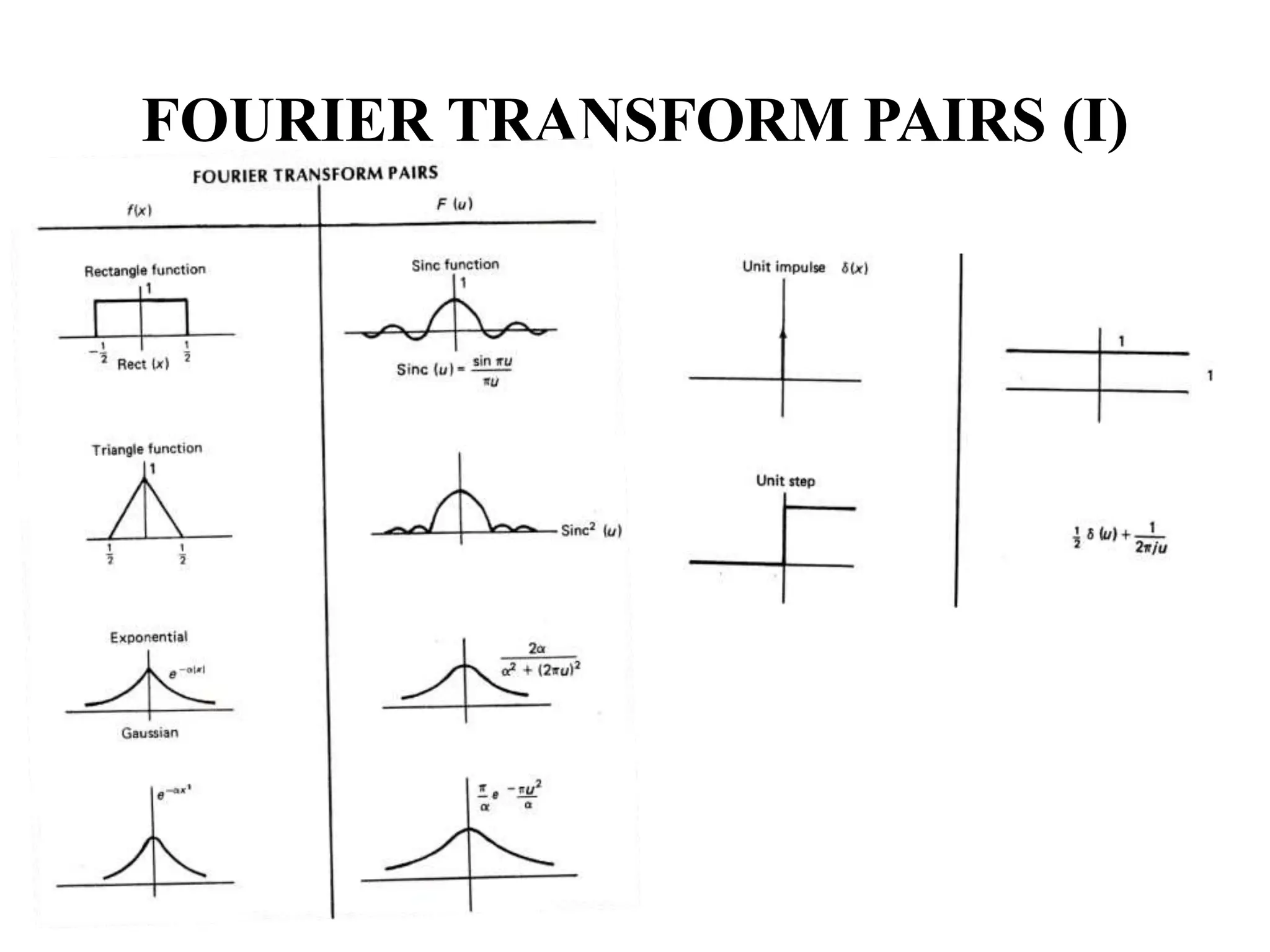
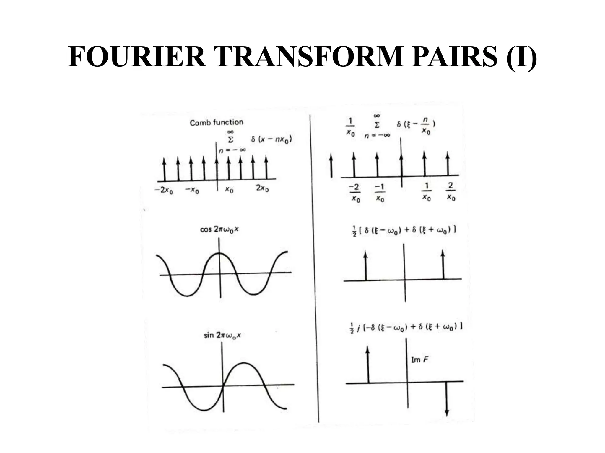
Explains Fourier Transform converting spatial domain to frequency domain; includes essential properties and transformation pairs.
Laplace Transform transitions time domain signals to complex frequency domain, describing properties of step and impulse functions.
Explores linearity, time shift, conditions for existence, including Dirichlet's conditions relevant for Laplace transforms.
Initial and final value theorems help determine signal behavior at extremes, addressing causality, stability, and systems.
Defines ROC for convergence of Laplace Transforms, characterizing based on signal types, including inverse transformations.
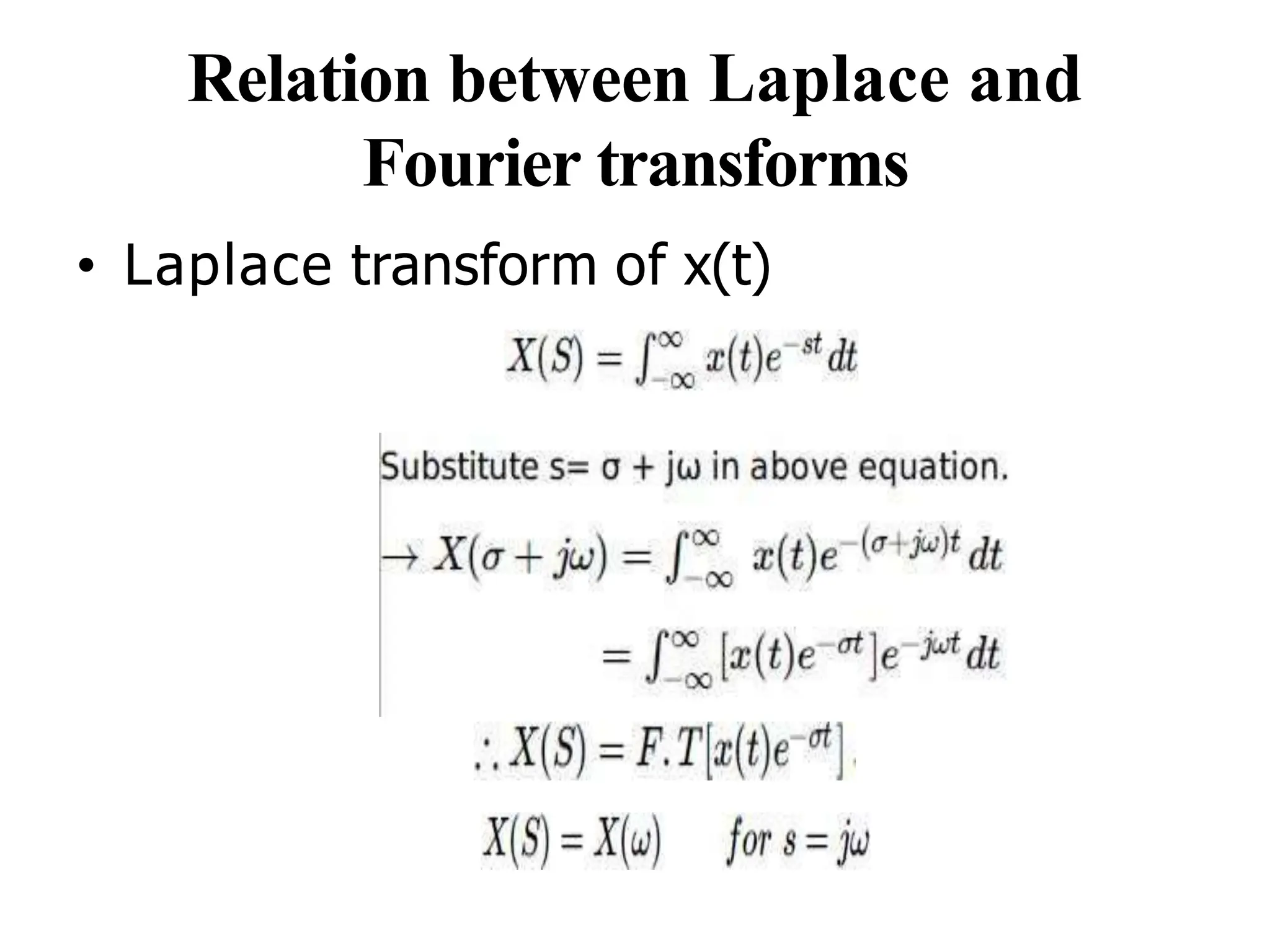
Explores the connection between Laplace and Fourier transforms, enhancing understanding of signal transformations.
SIGNAL
• Signal isa representation of physical quantity
(Sound, temperature, intensity, Pressure, etc..,) which
varies with respect to time or space or independent or
dependent variable.
• It is single valued function which carries information
by means Amplitude, Frequency and Phase.
• Example: voice signal, video signal, signals on
telephone wires etc.
4.
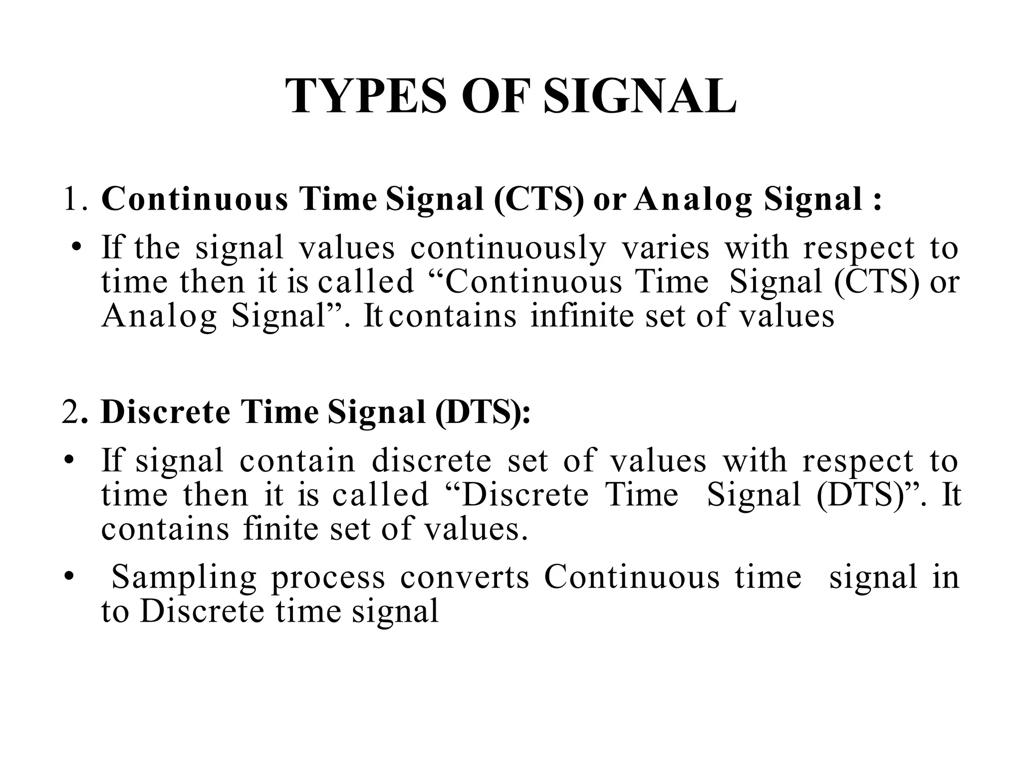
TYPES OF SIGNAL
1.Continuous Time Signal (CTS) or Analog Signal :
• If the signal values continuously varies with respect to
time then it is called “Continuous Time Signal (CTS) or
Analog Signal”. It contains infinite set of values
2. Discrete Time Signal (DTS):
• If signal contain discrete set of values with respect to
time then it is called “Discrete Time Signal (DTS)”. It
contains finite set of values.
• Sampling process converts Continuous time signal in
to Discrete time signal
5.
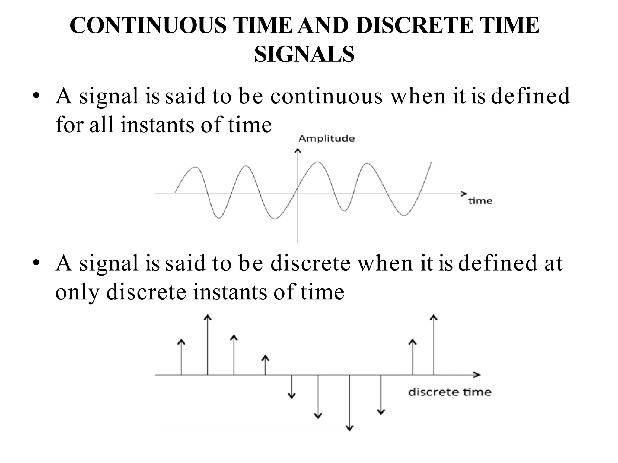
CONTINUOUS TIMEAND DISCRETETIME
SIGNALS
• A signal is said to be continuous when it is defined
for all instants of time
• A signal is said to be discrete when it is defined at
only discrete instants of time
6.
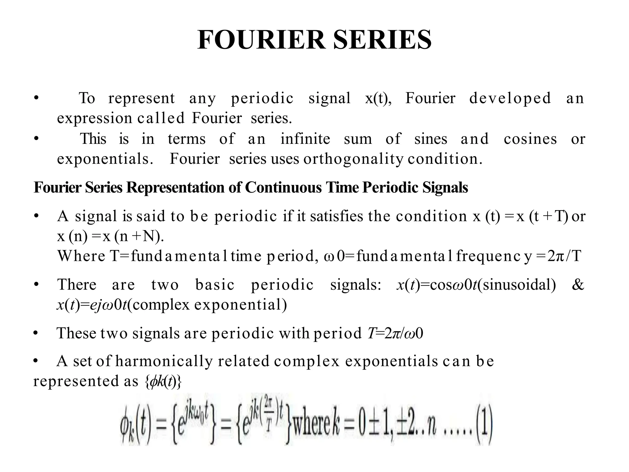
FOURIER SERIES
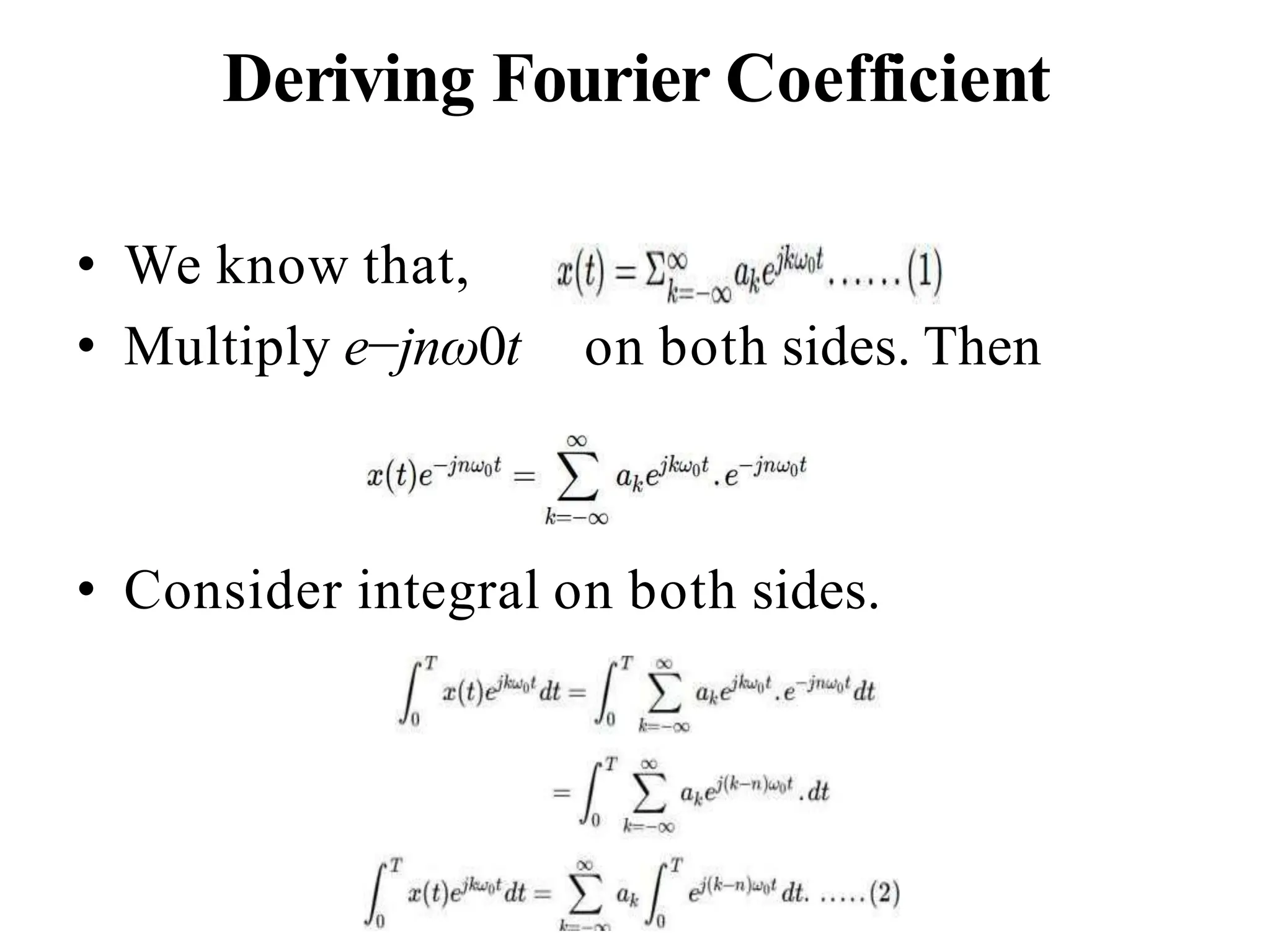
• Torepresent any periodic signal x(t), Fourier developed an
expression called Fourier series.
• This is in terms of an infinite sum of sines and cosines or
exponentials. Fourier series uses orthogonality condition.
Fourier Series Representation of Continuous Time Periodic Signals
• A signal is said to be periodic if it satisfies the condition x (t) =x (t +T) or
x (n) =x (n +N).
Where T=fund amenta l time period, ω0=fund amenta l frequenc y =2π/T
• There are two basic periodic signals: x(t)=cosω0t(sinusoidal) &
x(t)=ejω0t(complex exponential)
• These two signals are periodic with period T=2π/ω0
• A set of harmonically related complex exponentials can be
represented as {ϕk(t)}
7.
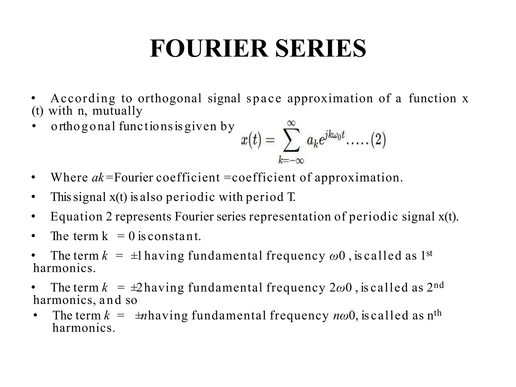
FOURIER SERIES
• Accordingto orthogonal signal space approximation of a function x
(t) with n, mutually
• orthogonal functionsisgiven by
• Where ak =Fourier coefficient =coefficient of approximation.
• Thissignal x(t) isalso periodic with period T.
• Equation 2 represents Fourier series representation of periodic signal x(t).
• The term k = 0 isconstant.
• The term k = ±1having fundamental frequency ω0 , is called as 1st
harmonics.
• The term k = ±2having fundamental frequency 2ω0 , is called as 2nd
harmonics, and so
• The term k = ±nhaving fundamental frequency nω0, iscalled as nth
harmonics.
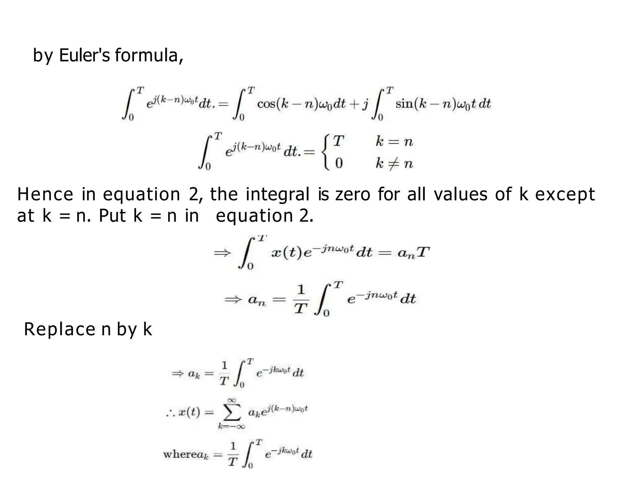
by Euler's formula,
Hencein equation 2, the integral is zero for all values of k except
at k = n. Put k = n in equation 2.
Replace n by k
10.
CT FOURIER SERIES– PROPERTIES
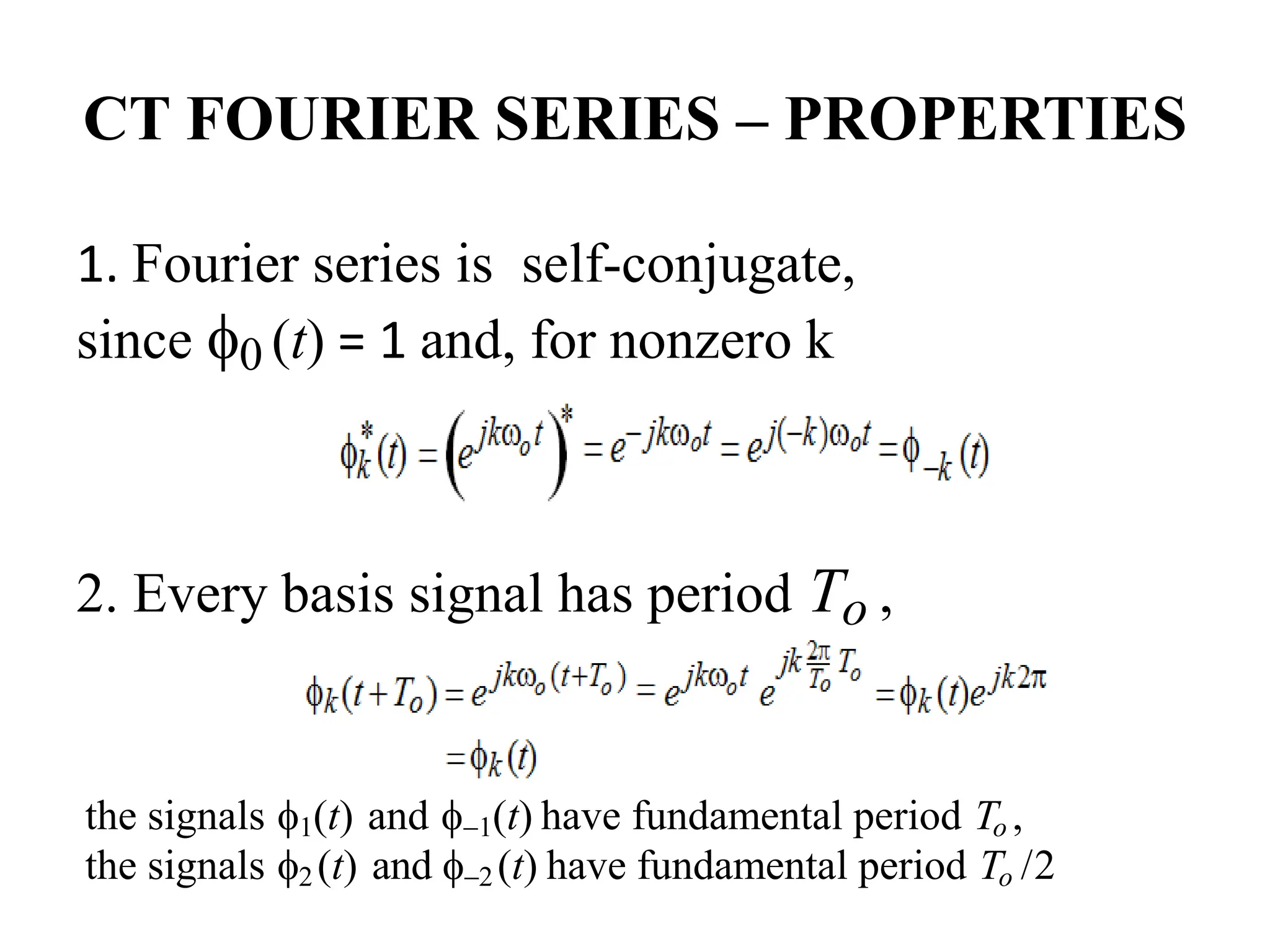
1. Fourier series is self-conjugate,
since 0 (t) = 1 and, for nonzero k
2. Every basis signal has period To ,
the signals 1(t) and 1(t) have fundamental period To ,
the signals 2 (t) and 2 (t) have fundamental period To /2
11.
CT FOURIER SERIES– PROPERTIES
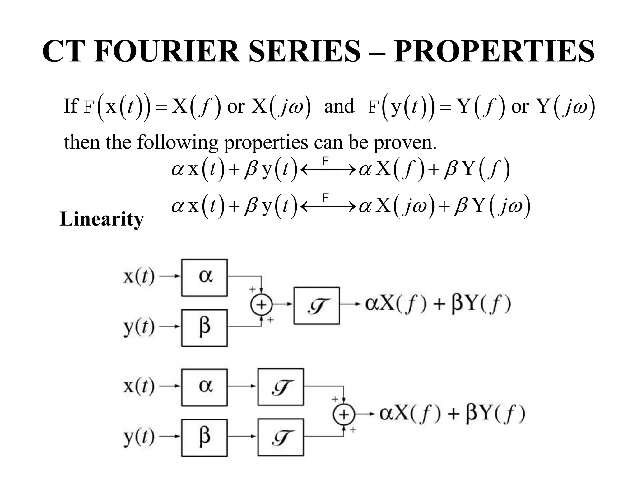
If x X or X and y Y or Y
then the following properties can be proven.
t f j t f j
F F
Linearity
x y X Y
x y X Y
t t f f
t t j j
F
F
12.
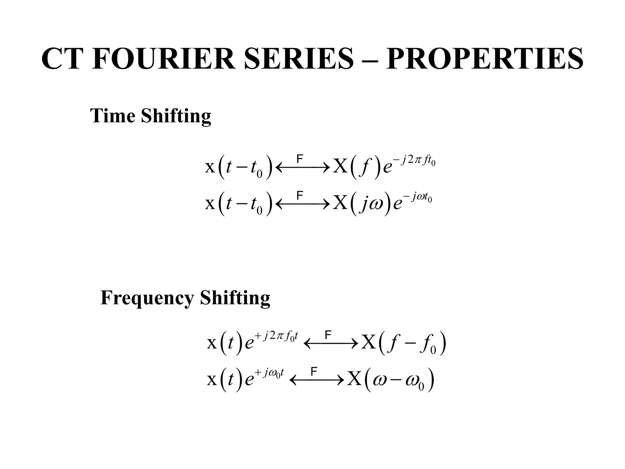
CT FOURIER SERIES– PROPERTIES
Time Shifting
0
0
2
0
0
x X
x X
j ft
j t
t t f e
t t j e
F
F
0
0
2
0
0
x X
x X
j f t
j t
t e f f
t e
F
F
Frequency Shifting
13.
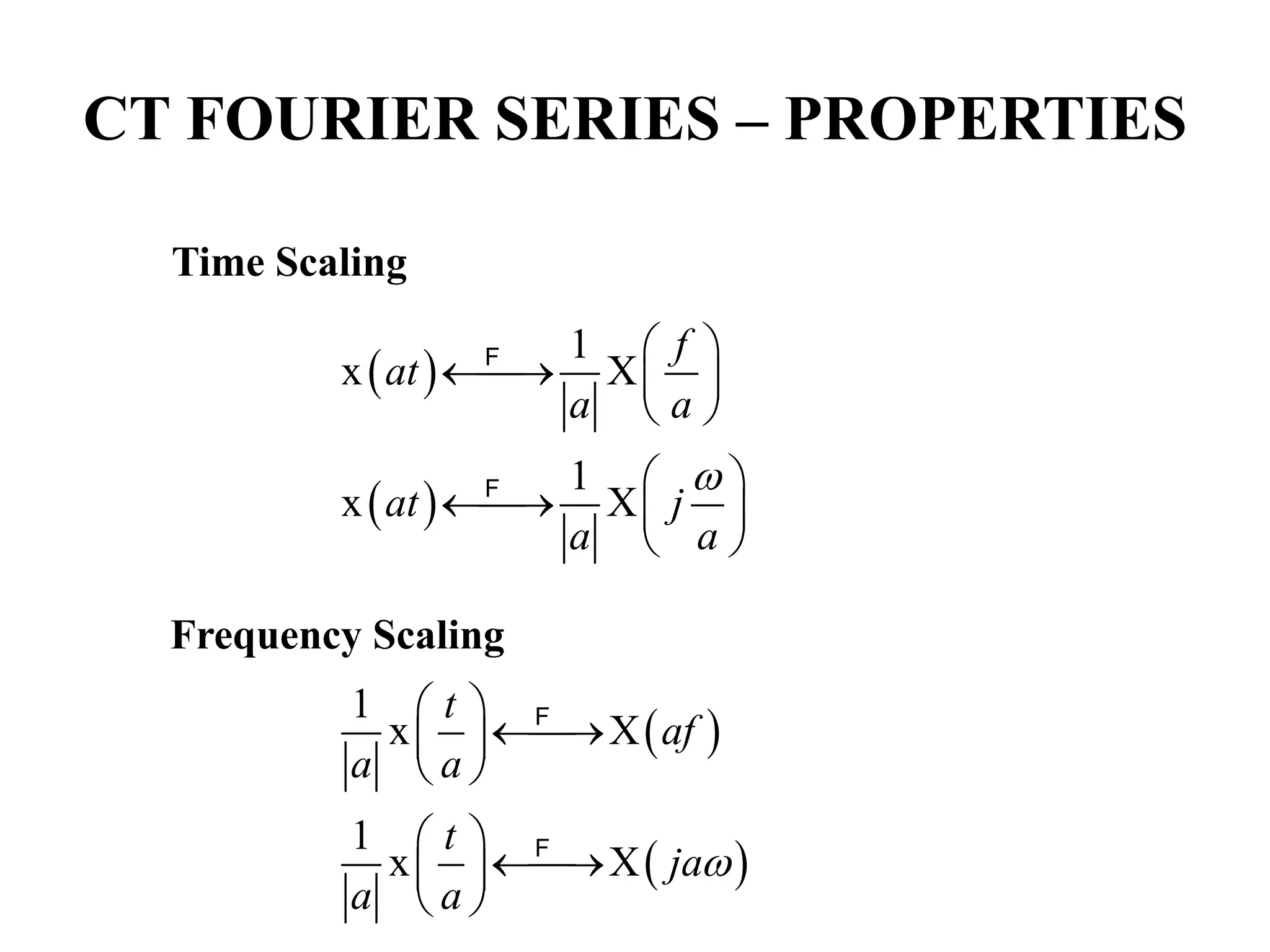
CT FOURIER SERIES– PROPERTIES
Time Scaling
1
x X
1
x X
f
at
a a
at j
a a
F
F
Frequency Scaling
1
x X
1
x X
t
af
a a
t
ja
a a
F
F
14.
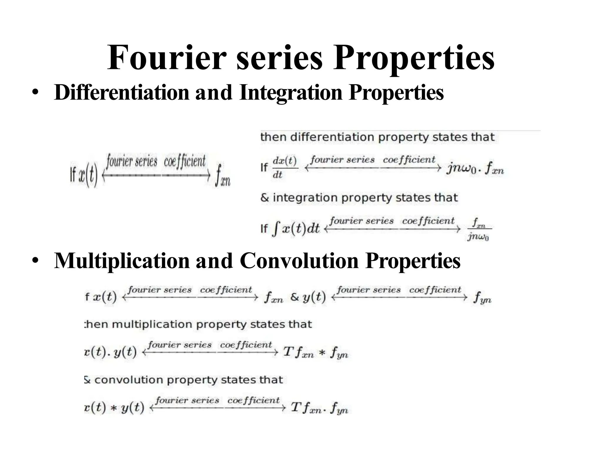
Fourier series Properties
•Differentiation and Integration Properties
• Multiplication and Convolution Properties
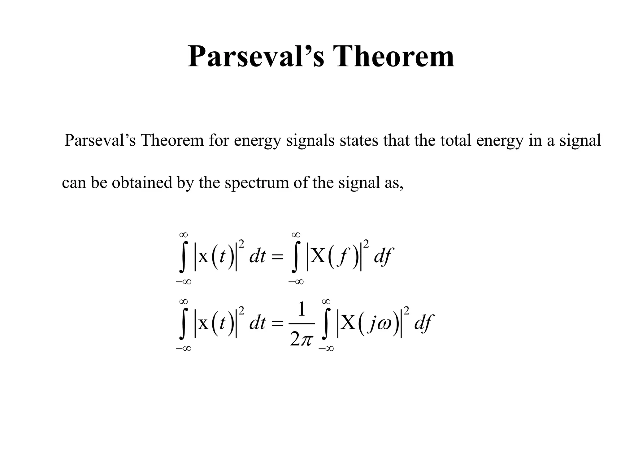
Parseval’s Theorem
Parseval’s Theoremfor energy signals states that the total energy in a signal
can be obtained by the spectrum of the signal as,
2 2
2 2
x X
1
x X
2
t dt f df
t dt j df
17.
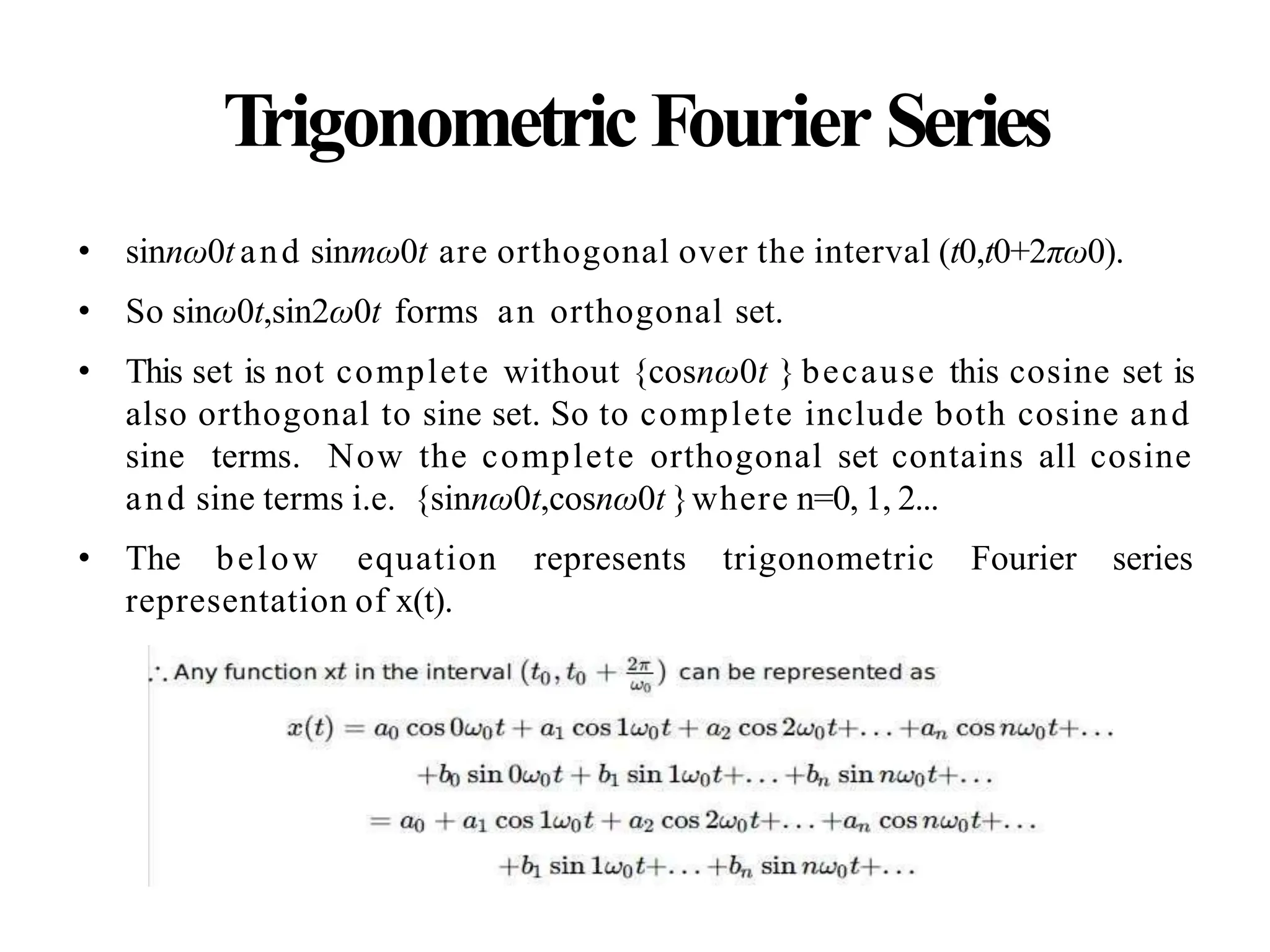
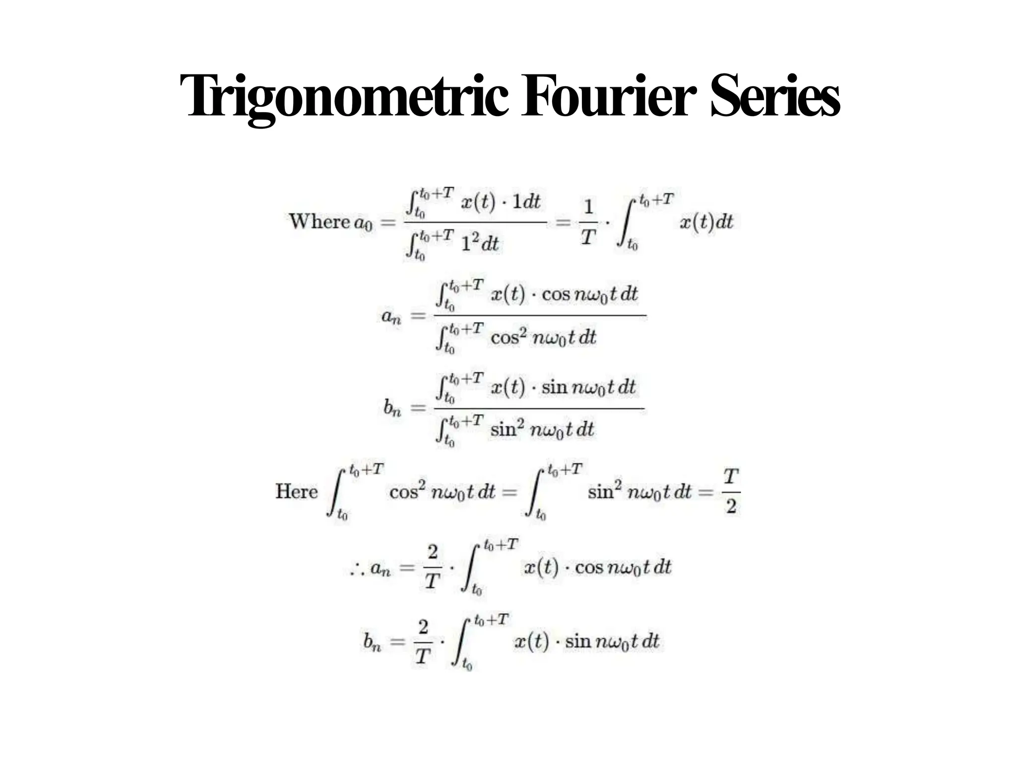
Trigonometric Fourier Series
•sinnω0t and sinmω0t are orthogonal over the interval (t0,t0+2πω0).
• So sinω0t,sin2ω0t forms an orthogonal set.
• This set is not complete without {cosnω0t } because this cosine set is
also orthogonal to sine set. So to complete include both cosine and
sine terms. Now the complete orthogonal set contains all cosine
and sine terms i.e. {sinnω0t,cosnω0t }where n=0, 1, 2...
• The below equation represents trigonometric Fourier series
representation of x(t).
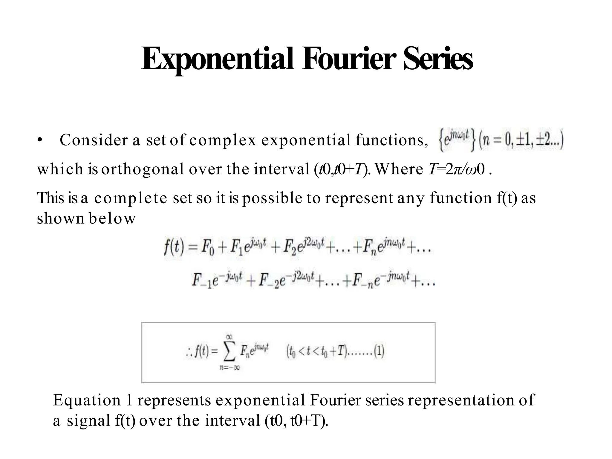
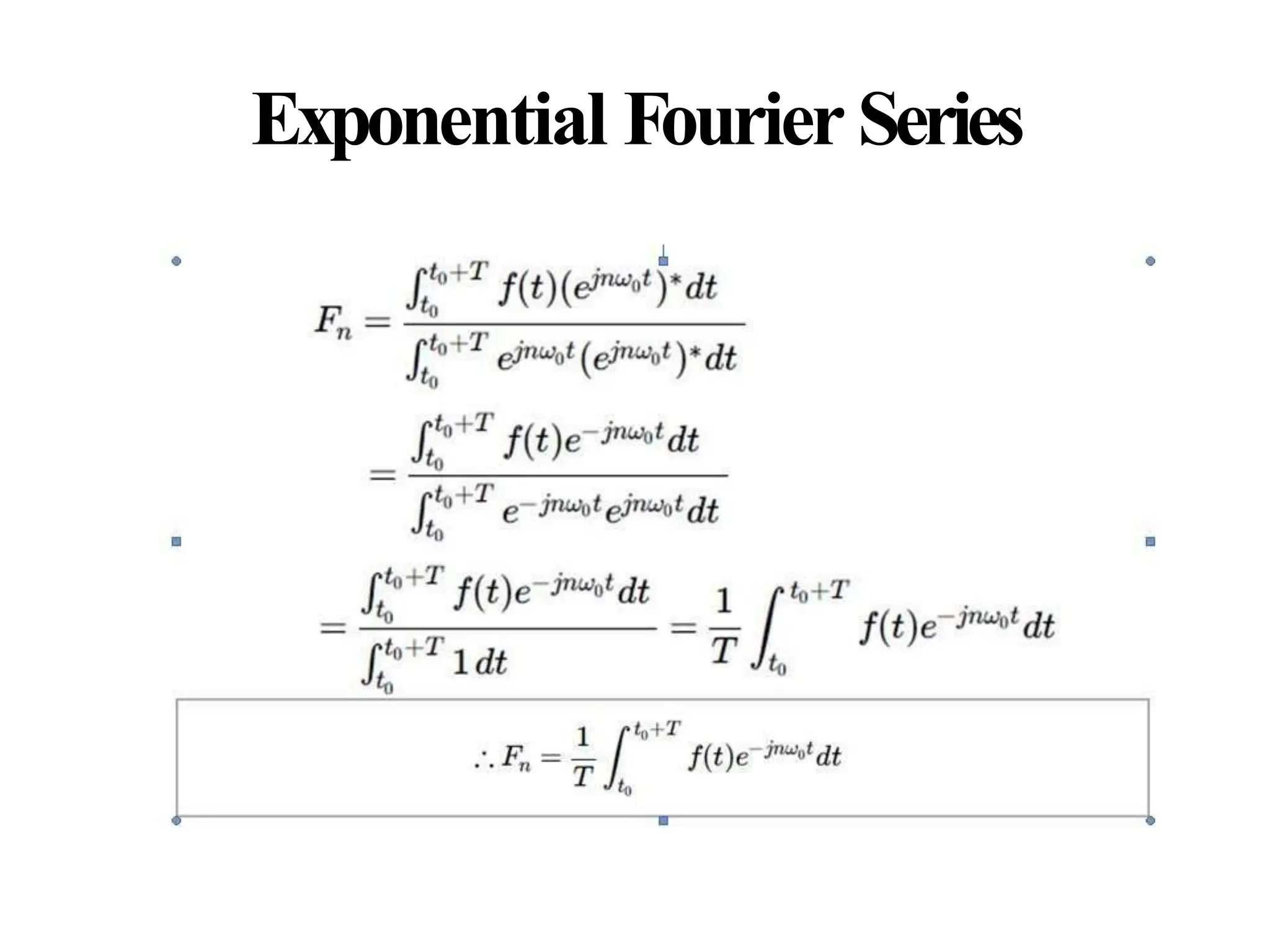
Exponential Fourier Series
•Consider a set of complex exponential functions,
which is orthogonal over the interval (t0,t0+T).Where T=2π/ω0 .
This is a complete set so it is possible to represent any function f(t) as
shown below
Equation 1 represents exponential Fourier series representation of
a signal f(t) over the interval (t0, t0+T).
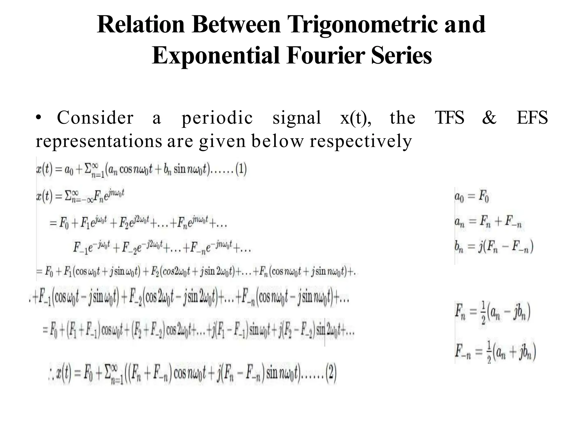
Relation Between Trigonometricand
Exponential Fourier Series
• Consider a periodic signal x(t), the TFS & EFS
representations are given below respectively
22.
CONTINUOS TIME FOURIERTRANSFORM
• The main drawback of Fourier series is, it is only applicable to periodic
signals.
• There are some naturally produced signals such as nonperiodic or
aperiodic, which cannot be represented using Fourier series.
• To overcome this shortcoming, Fourier developed a mathematical
model to transform signals between time (or spatial) domain to
frequency domain & vice versa, which is called 'Fourier transform'.
• Fourier transform has many applications in physics and engineering
such as analysis of L
TI systems, RADAR, astronomy, signal processing
etc.
23.
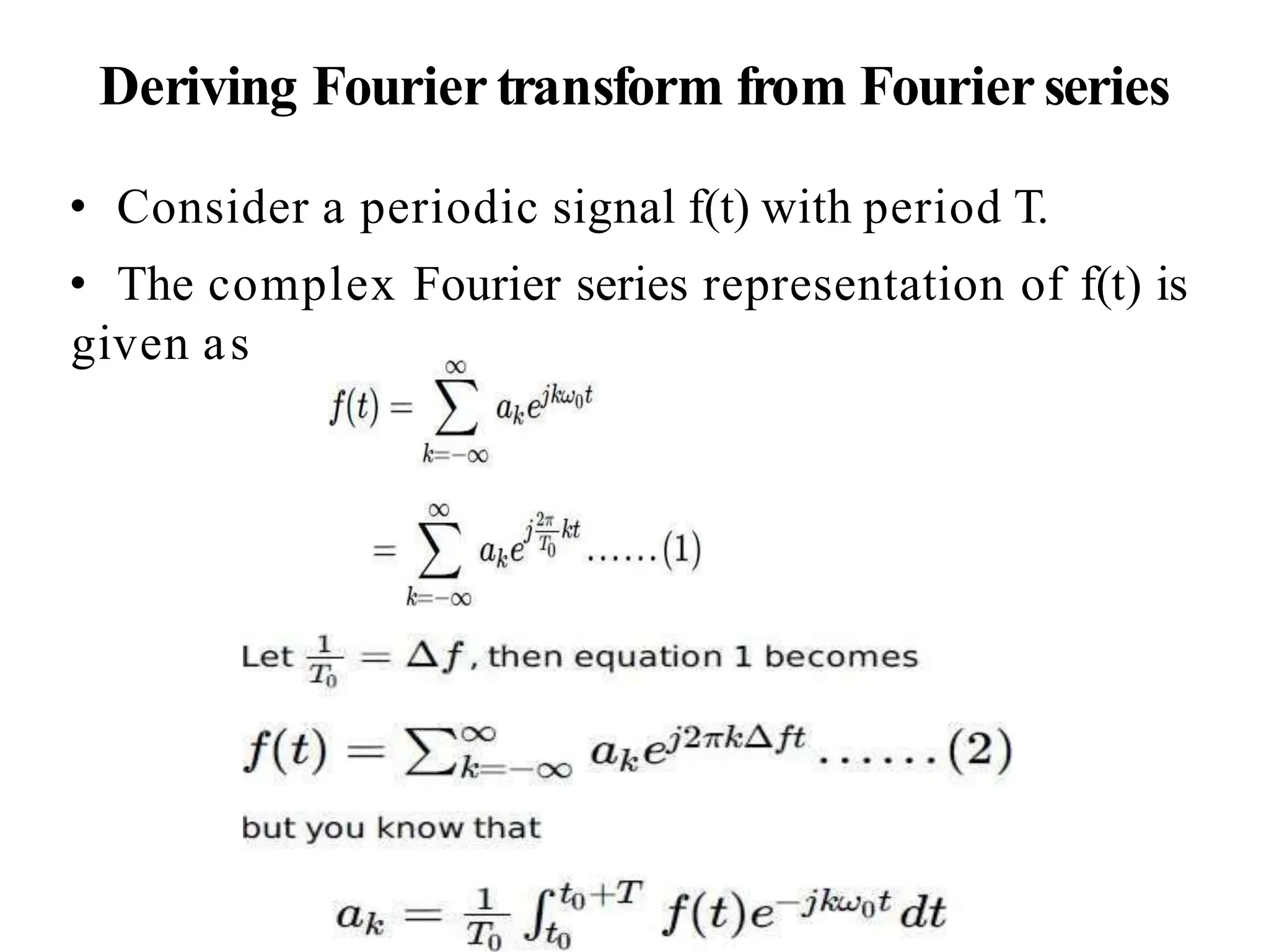
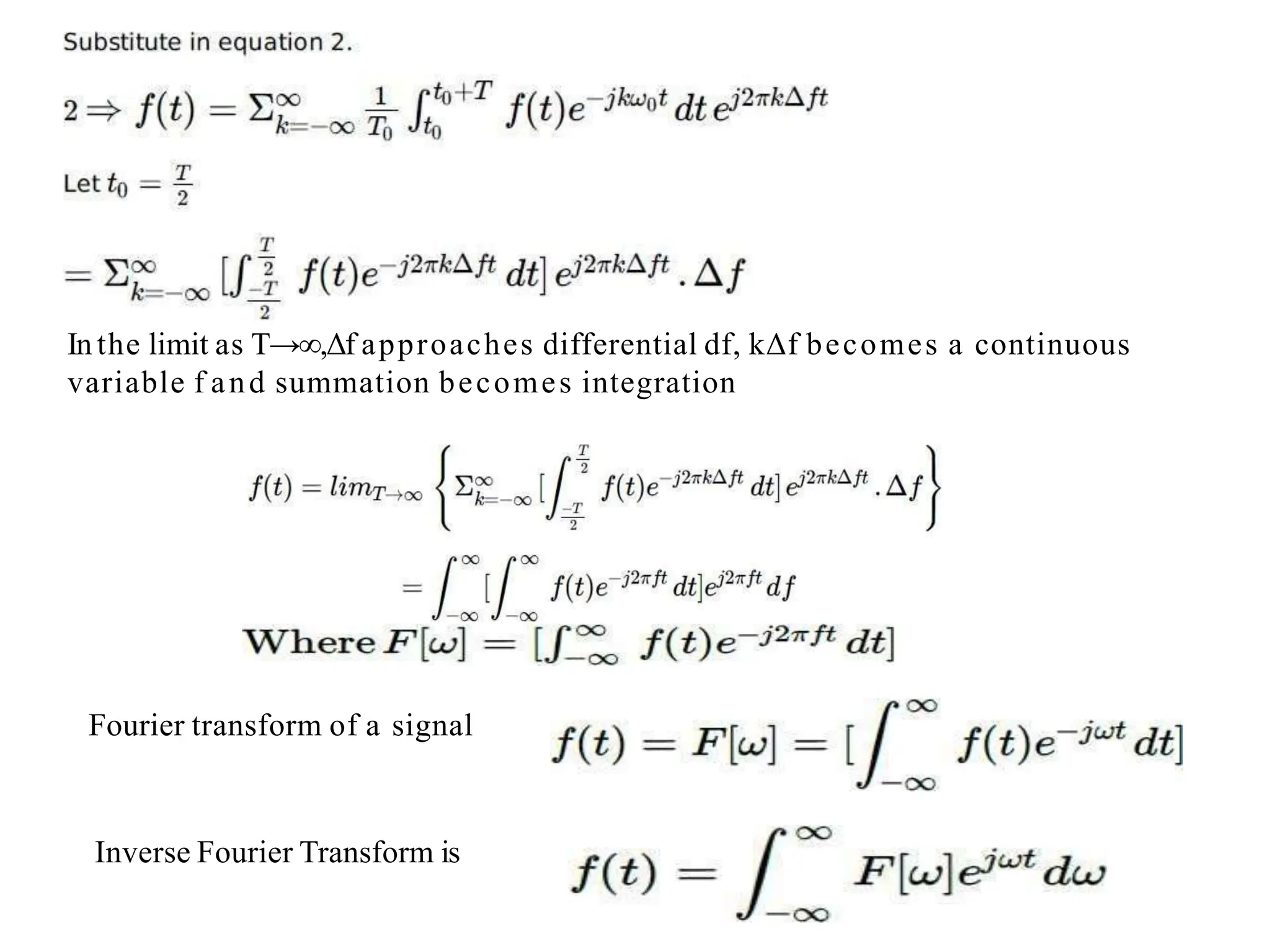
Deriving Fourier transformfrom Fourier series
• Consider a periodic signal f(t) with period T.
• The complex Fourier series representation of f(t) is
given as
24.
In the limitas T→∞,Δf approaches differential df, kΔf becomes a continuous
variable f and summation becomes integration
Fourier transform of a signal
Inverse Fourier Transform is
25.
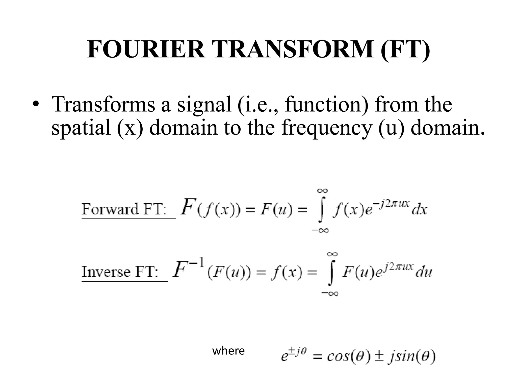
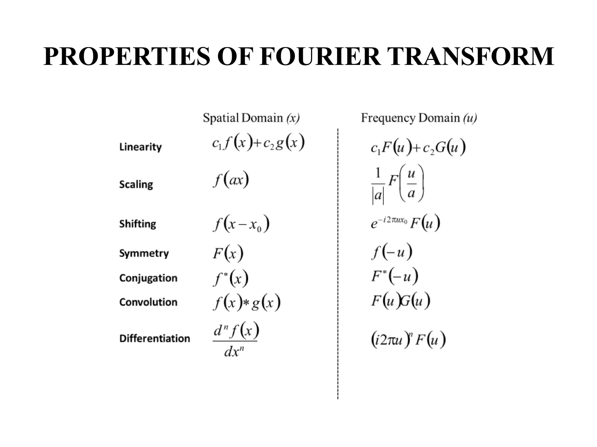
FOURIER TRANSFORM (FT)
•Transforms a signal (i.e., function) from the
spatial (x) domain to the frequency (u) domain.
where
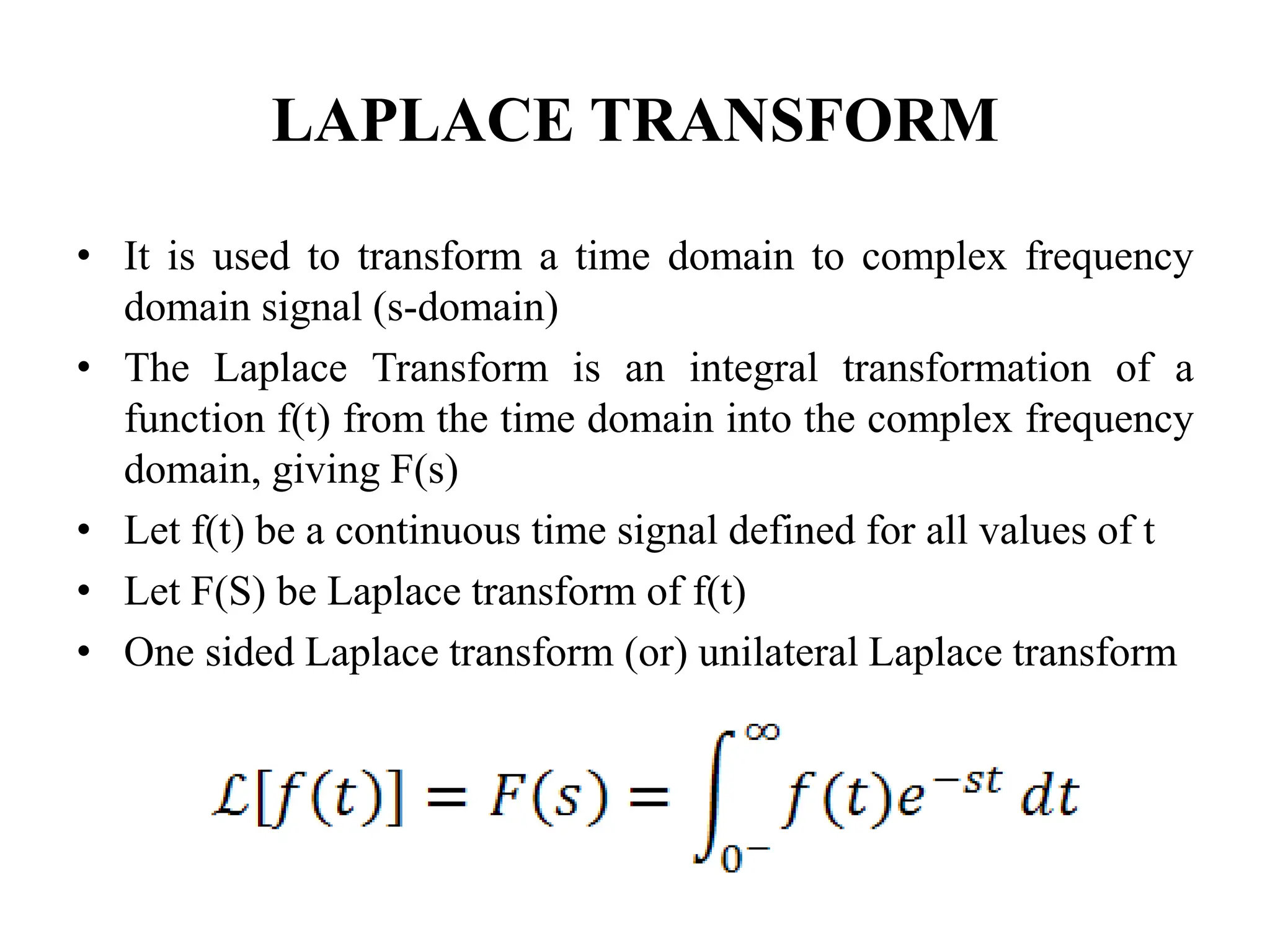
LAPLACE TRANSFORM
• Itis used to transform a time domain to complex frequency
domain signal (s-domain)
• The Laplace Transform is an integral transformation of a
function f(t) from the time domain into the complex frequency
domain, giving F(s)
• Let f(t) be a continuous time signal defined for all values of t
• Let F(S) be Laplace transform of f(t)
• One sided Laplace transform (or) unilateral Laplace transform
30.
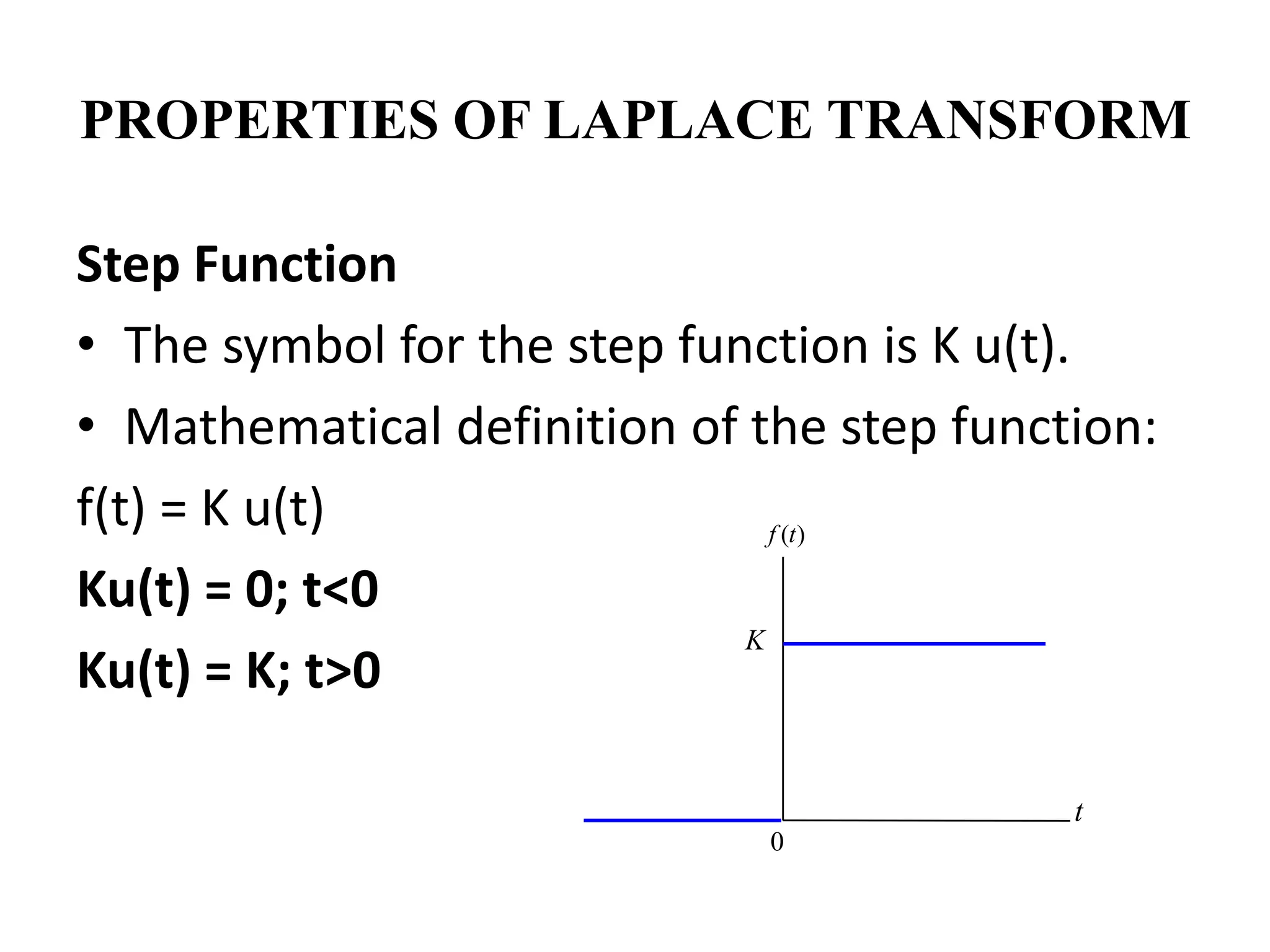
PROPERTIES OF LAPLACETRANSFORM
Step Function
• The symbol for the step function is K u(t).
• Mathematical definition of the step function:
f(t) = K u(t)
Ku(t) = 0; t<0
Ku(t) = K; t>0
)
(t
f
K
0
t
31.
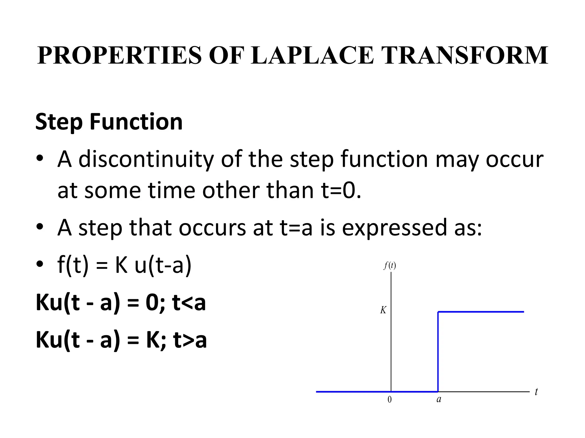
PROPERTIES OF LAPLACETRANSFORM
Step Function
• A discontinuity of the step function may occur
at some time other than t=0.
• A step that occurs at t=a is expressed as:
• f(t) = K u(t-a)
Ku(t - a) = 0; t<a
Ku(t - a) = K; t>a
)
(t
f
K
t
a
0
32.
PROPERTIES OF LAPLACETRANSFORM
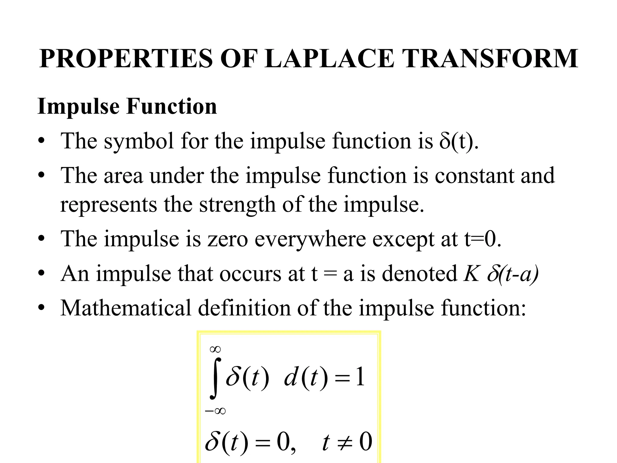
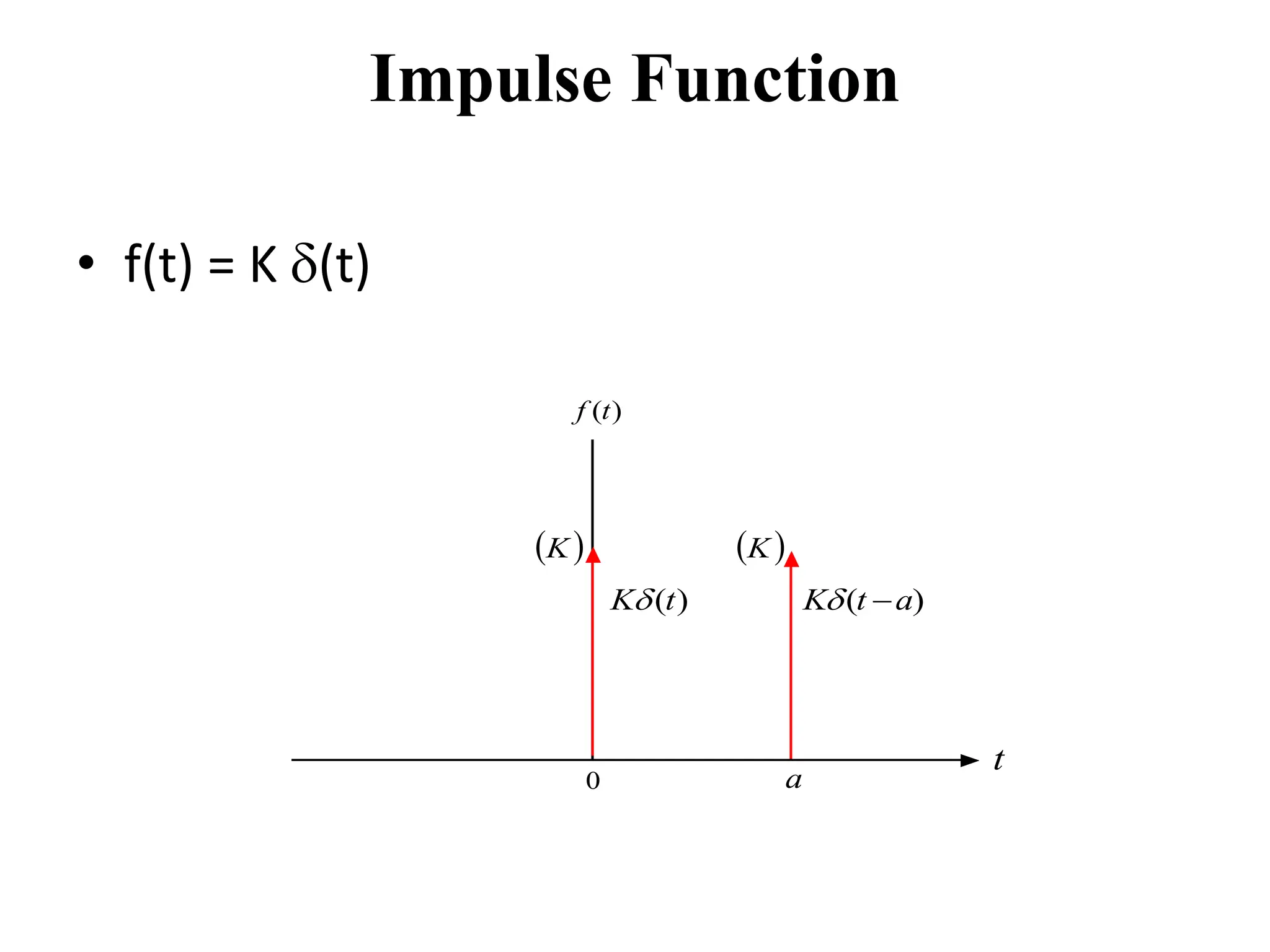
Impulse Function
• The symbol for the impulse function is (t).
• The area under the impulse function is constant and
represents the strength of the impulse.
• The impulse is zero everywhere except at t=0.
• An impulse that occurs at t = a is denoted K (t-a)
• Mathematical definition of the impulse function:
0
,
0
)
(
1
)
(
)
(
t
t
t
d
t
PROPERTIES OF LAPLACETRANSFORM
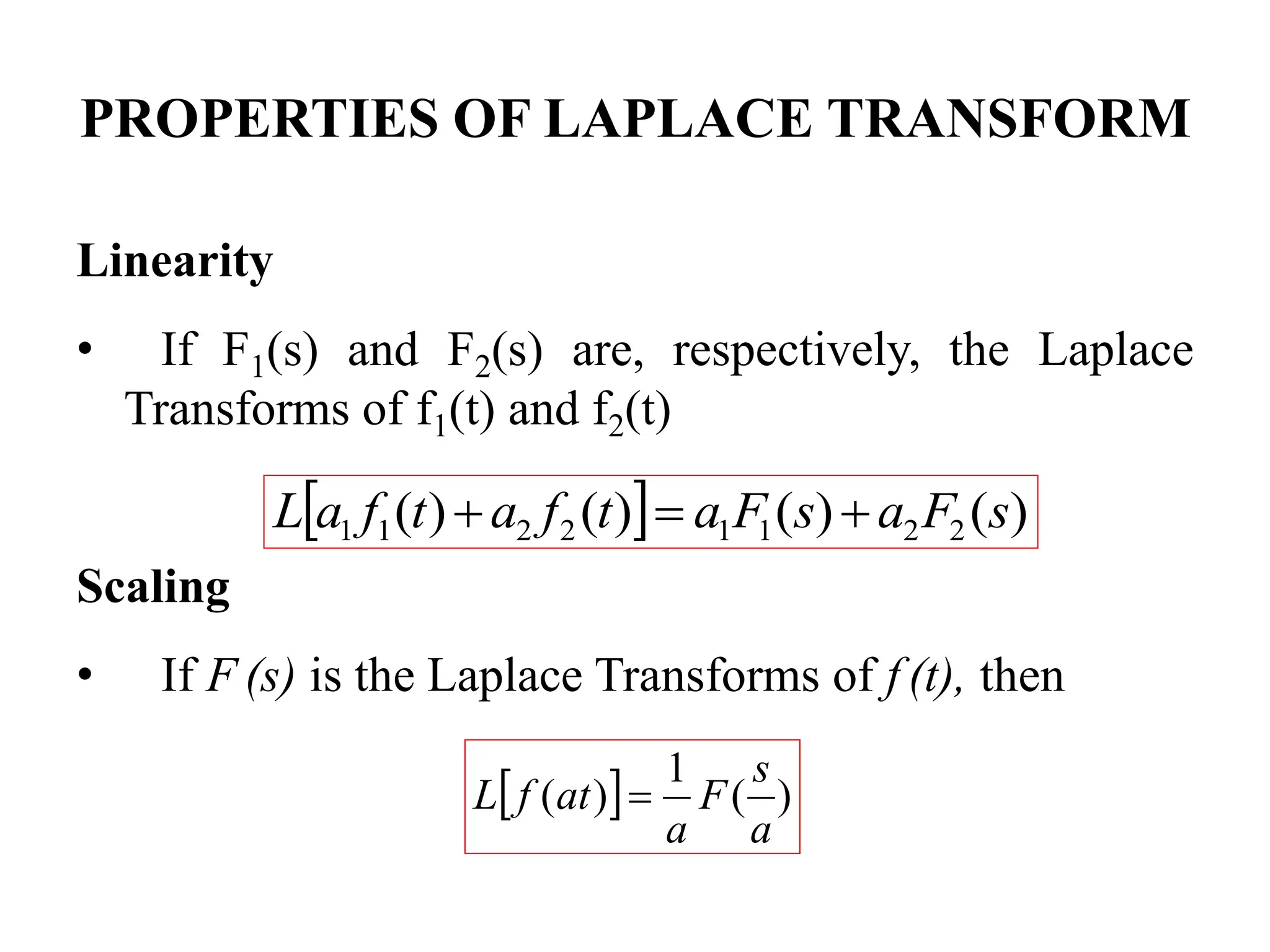
Linearity
• If F1(s) and F2(s) are, respectively, the Laplace
Transforms of f1(t) and f2(t)
Scaling
• If F (s) is the Laplace Transforms of f (t), then
)
(
)
(
)
(
)
( 2
2
1
1
2
2
1
1 s
F
a
s
F
a
t
f
a
t
f
a
L
)
(
1
)
(
a
s
F
a
at
f
L
35.
PROPERTIES OF LAPLACETRANSFORM
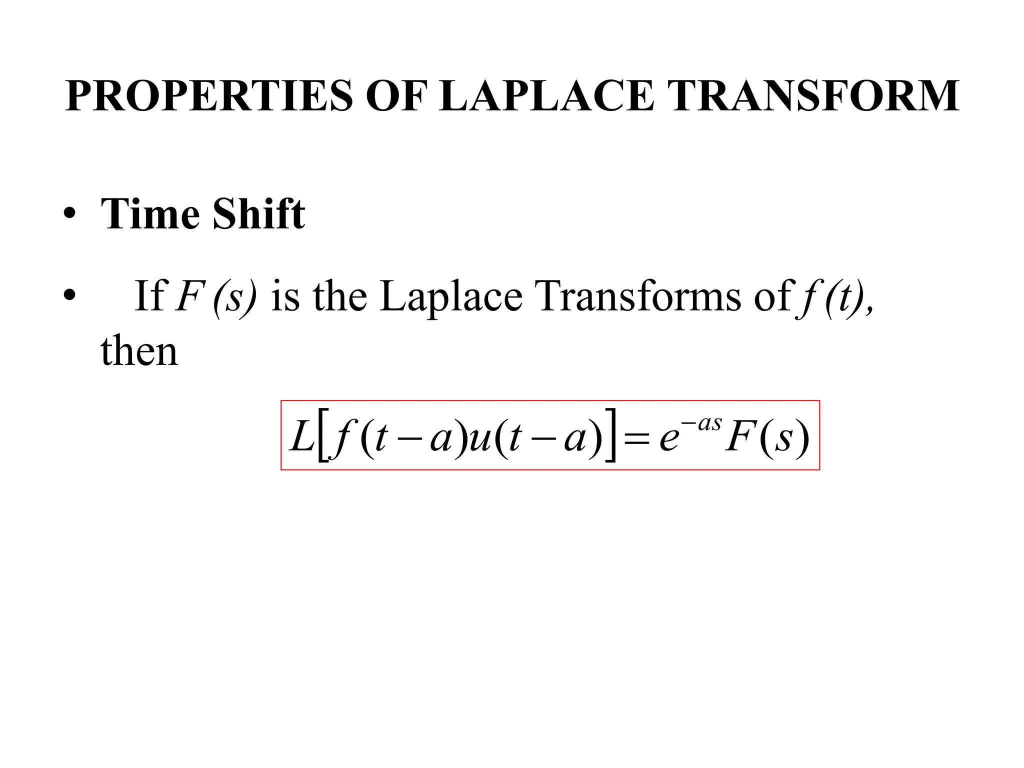
• Time Shift
• If F (s) is the Laplace Transforms of f (t),
then
)
(
)
(
)
( s
F
e
a
t
u
a
t
f
L as
36.
Conditions for Existenceof Laplace Transform
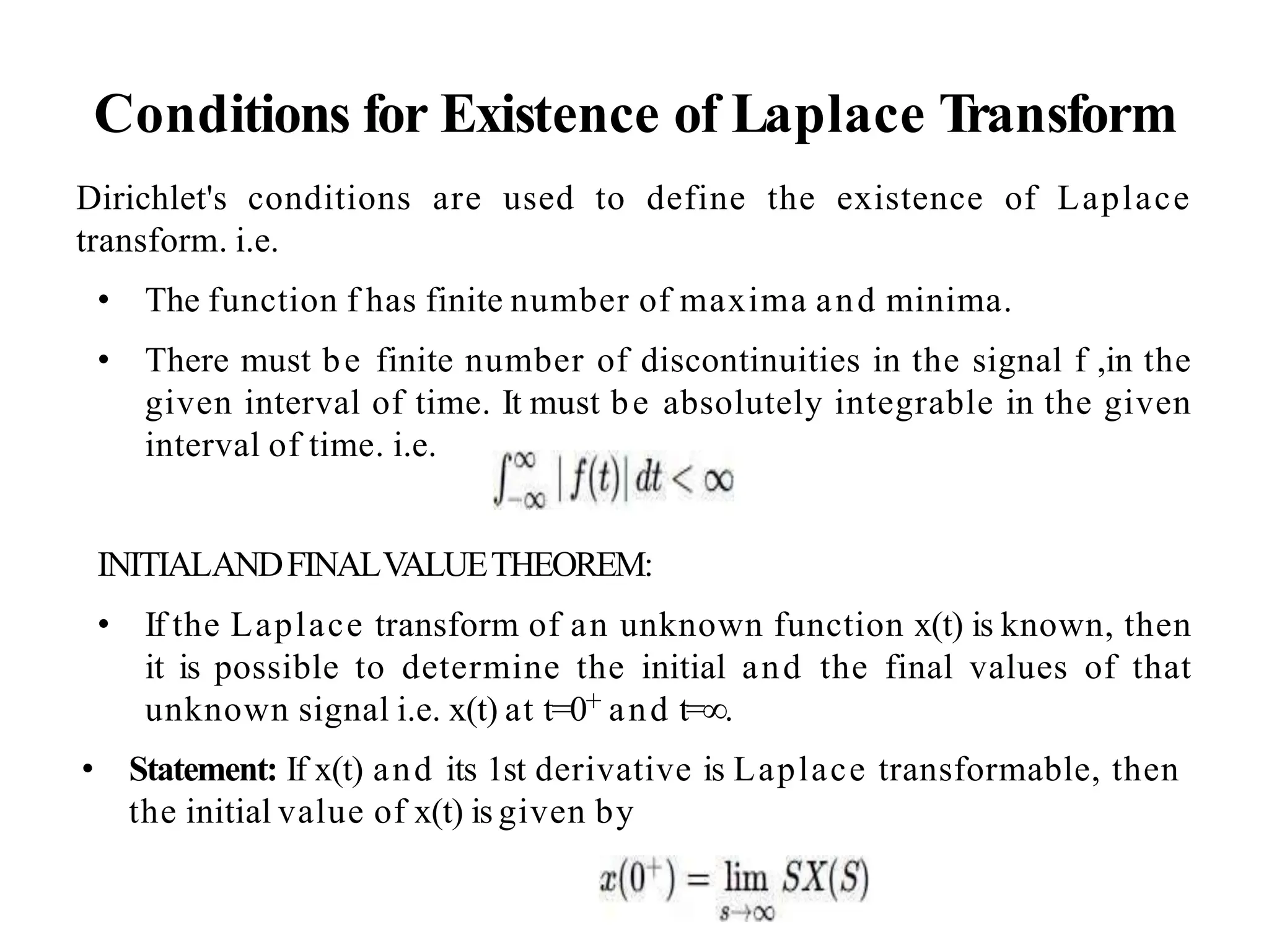
Dirichlet's conditions are used to define the existence of Laplace
transform. i.e.
• The function f has finite number of maxima and minima.
• There must be finite number of discontinuities in the signal f ,in the
given interval of time. It must be absolutely integrable in the given
interval of time. i.e.
INITIALANDFINALVALUETHEOREM:
• If the Laplace transform of an unknown function x(t) is known, then
it is possible to determine the initial and the final values of that
unknown signal i.e. x(t) at t=0+ and t=∞.
• Statement: If x(t) and its 1st derivative is Laplace transformable, then
the initial value of x(t) is given by
37.
DIRICHLET CONDITION
Theorem
If x(t)is periodic with fundamental period To ,
The Dirichlet conditions:
(1) x(t) is a periodic function;
(2) x(t) has only a finite number of finite discontinuities;
(3) x(t) has only a finite number of extrem values, maxima and minima in the
interval [0,2].
Then
(i) limK (I2K 1) 0 ,
(ii) at each value of t where x(t) is continuous, x(t)
(iii) at each value of t where x(t) has a discontinuity,
takes the value of the mid-point of the discontinuity.
• The Dirichlet condition is a sufficient condition for a type of convergence of the Fourier
series.
• The nature of convergence of Fourier series results in an important phenomenon called
the Gibbs Effect when a truncated (finite) Fourier series is used as an approximation to
the signal.
38.
INITIALAND FINAL VALUETHEOREMS
• Theorem:
• Proof: Applying the differentiation property:
Theorem)
Value
(Final
)
(
lim
)
x(
Theorem)
Value
(Initial
)
(
lim
)
0
(
0
s
sX
s
sX
x
s
s
)
(
lim
)
(
0
)
0
(
)
(
)
0
(
)
(
)
(
lim
)
0
(
0
)
0
(
)
(
:
two
the
Combining
0
)
0
(
)
(
)
1
(
)
(
0
)
0
(
)
(
)
(
)
(
)
0
(
)
(
)
(
0
0
0
0
s
sX
x
s
x
s
sX
x
x
s
sX
x
s
x
s
sX
s
x
x
dt
dt
t
dx
s
dt
dt
t
dx
dt
e
dt
t
dx
dt
t
dx
x
s
sX
dt
t
dx
s
s
st
UL
UL
• The initial value theorem can be extended to higher-order derivatives:
• Allow initial and final conditions to be computed directly from the transform.
)]
0
(
)
(
[
lim
)
( 2
0
sx
s
X
s
dt
t
dx
s
t
39.
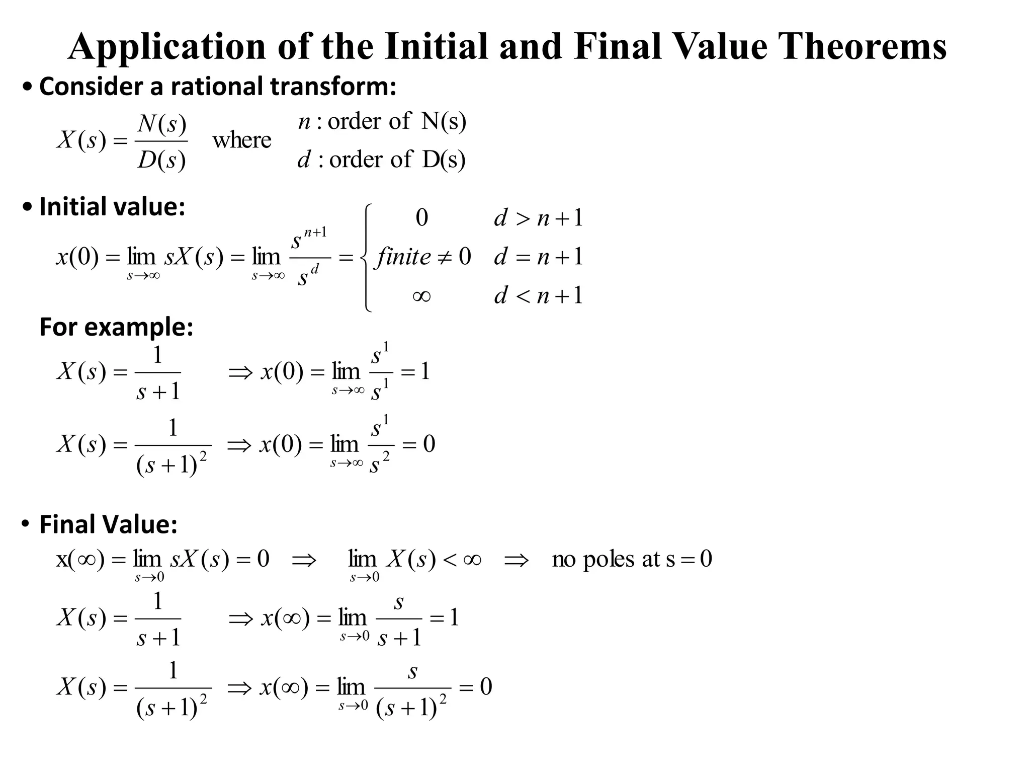
Application of theInitial and Final Value Theorems
• Consider a rational transform:
• Initial value:
For example:
• Final Value:
D(s)
of
order
:
N(s)
of
order
:
where
)
(
)
(
)
(
d
n
s
D
s
N
s
X
1
1
1
0
0
lim
)
(
lim
)
0
(
1
n
d
n
d
n
d
finite
s
s
s
sX
x d
n
s
s
0
lim
)
0
(
)
1
(
1
)
(
1
lim
)
0
(
1
1
)
(
2
1
2
1
1
s
s
x
s
s
X
s
s
x
s
s
X
s
s
0
s
at
poles
no
)
(
lim
0
)
(
lim
)
x(
0
0
s
X
s
sX
s
s
0
)
1
(
lim
)
(
)
1
(
1
)
(
1
1
lim
)
(
1
1
)
(
2
0
2
0
s
s
x
s
s
X
s
s
x
s
s
X
s
s
40.
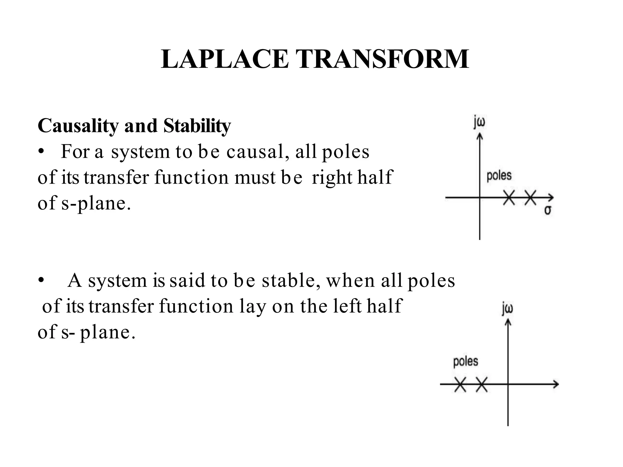
LAPLACE TRANSFORM
Causality andStability
• For a system to be causal, all poles
of its transfer function must be right half
of s-plane.
• A system is said to be stable, when all poles
of its transfer function lay on the left half
of s- plane.
41.
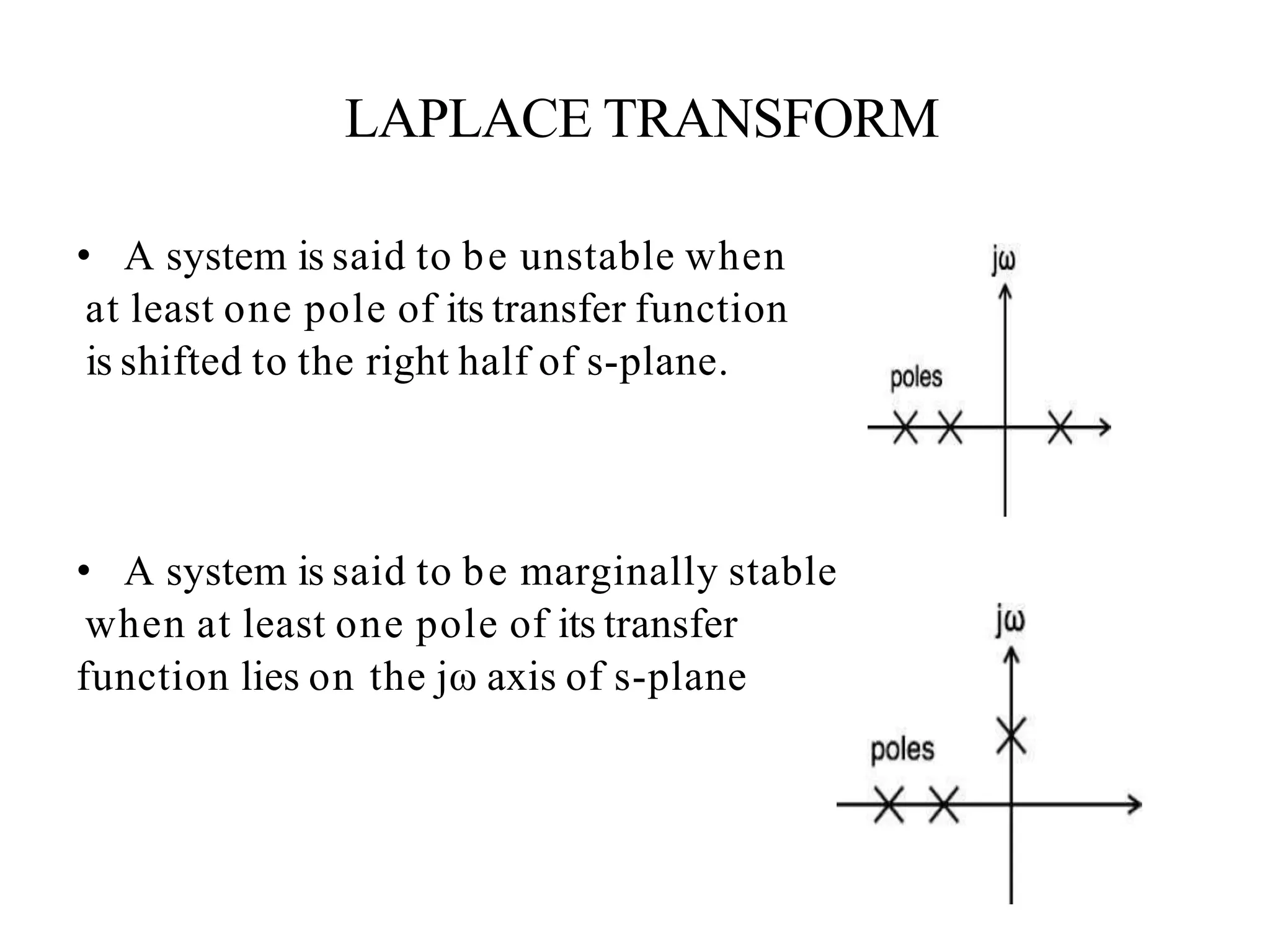
LAPLACE TRANSFORM
• Asystem is said to be unstable when
at least one pole of its transfer function
is shifted to the right half of s-plane.
• A system is said to be marginally stable
when at least one pole of its transfer
function lies on the jω axis of s-plane
42.
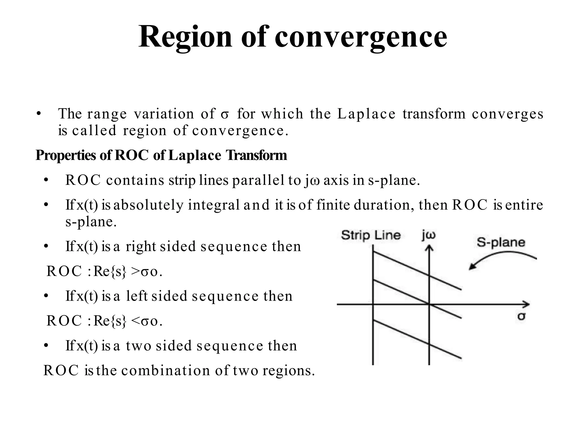
Region of convergence
•The range variation of σ for which the Laplace transform converges
is called region of convergence.
Properties of ROC of Laplace Transform
• ROC contains strip lines parallel to jω axis in s-plane.
• Ifx(t) is absolutely integral and it is of finite duration, then ROC is entire
s-plane.
• Ifx(t) is a right sided sequence then
ROC :Re{s} >σo.
• Ifx(t) is a left sided sequence then
ROC :Re{s} <σo.
• Ifx(t) is a two sided sequence then
ROC isthe combination of two regions.
43.
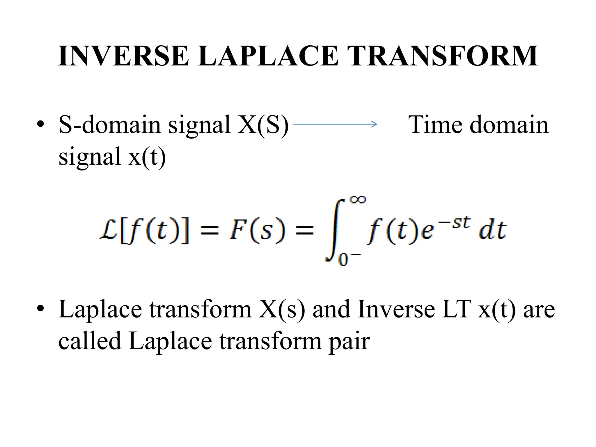
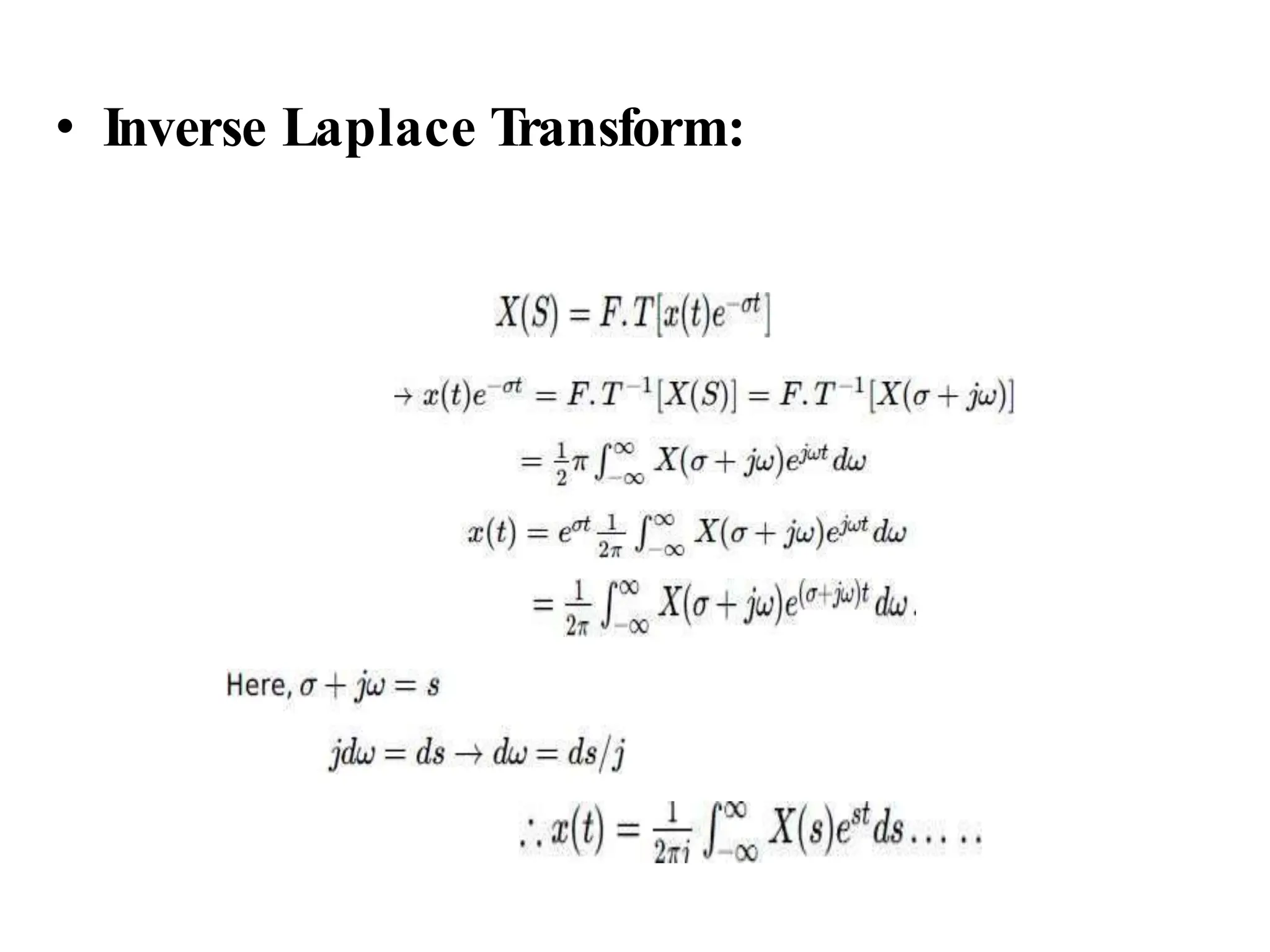
INVERSE LAPLACE TRANSFORM
•S-domain signal X(S) Time domain
signal x(t)
• Laplace transform X(s) and Inverse LT x(t) are
called Laplace transform pair
![DIRICHLET CONDITION
Theorem
If x(t) is periodic with fundamental period To ,
The Dirichlet conditions:
(1) x(t) is a periodic function;
(2) x(t) has only a finite number of finite discontinuities;
(3) x(t) has only a finite number of extrem values, maxima and minima in the
interval [0,2].
Then
(i) limK (I2K 1) 0 ,
(ii) at each value of t where x(t) is continuous, x(t)
(iii) at each value of t where x(t) has a discontinuity,
takes the value of the mid-point of the discontinuity.
• The Dirichlet condition is a sufficient condition for a type of convergence of the Fourier
series.
• The nature of convergence of Fourier series results in an important phenomenon called
the Gibbs Effect when a truncated (finite) Fourier series is used as an approximation to
the signal.](https://image.slidesharecdn.com/ssunit2-240402184746-bf85a6cb/75/Signals-and-Systems-Fourier-Series-and-Transform-37-2048.jpg)
![INITIALAND FINAL VALUE THEOREMS
• Theorem:
• Proof: Applying the differentiation property:
Theorem)
Value
(Final
)
(
lim
)
x(
Theorem)
Value
(Initial
)
(
lim
)
0
(
0
s
sX
s
sX
x
s
s
)
(
lim
)
(
0
)
0
(
)
(
)
0
(
)
(
)
(
lim
)
0
(
0
)
0
(
)
(
:
two
the
Combining
0
)
0
(
)
(
)
1
(
)
(
0
)
0
(
)
(
)
(
)
(
)
0
(
)
(
)
(
0
0
0
0
s
sX
x
s
x
s
sX
x
x
s
sX
x
s
x
s
sX
s
x
x
dt
dt
t
dx
s
dt
dt
t
dx
dt
e
dt
t
dx
dt
t
dx
x
s
sX
dt
t
dx
s
s
st
UL
UL
• The initial value theorem can be extended to higher-order derivatives:
• Allow initial and final conditions to be computed directly from the transform.
)]
0
(
)
(
[
lim
)
( 2
0
sx
s
X
s
dt
t
dx
s
t
](https://image.slidesharecdn.com/ssunit2-240402184746-bf85a6cb/75/Signals-and-Systems-Fourier-Series-and-Transform-38-2048.jpg)