Downloaded 899 times
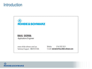
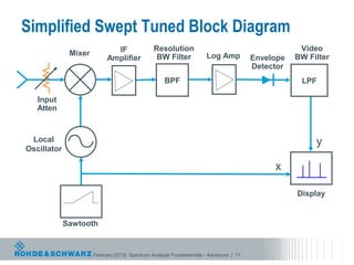
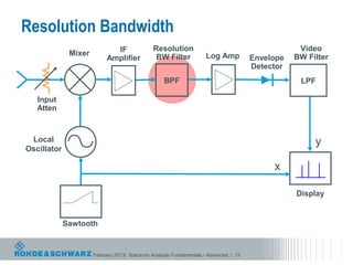
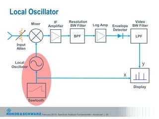
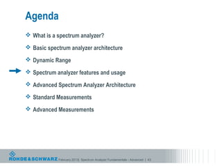
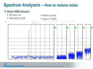
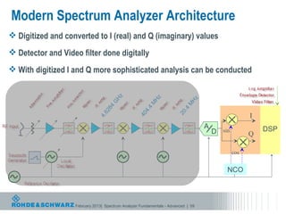
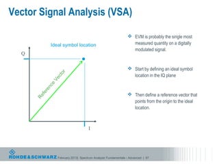
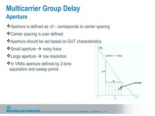
![Measuring Noise: Sample Detector w/Log Averaging
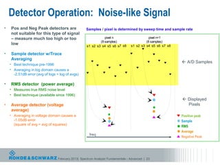
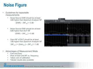
• Video (log) averaging (dBm) values causes a negative shift in the result.
• Positive peaks are compressed Avg value of a Gaussian variable g(x) with µ = 0, σ = 1
• Negative peaks are enhanced → E [ 20 log( g ( x ) ) ] = −2.51 dB
• The log of the average is not the same as the average of the log values
• The delta for a Gaussian distribution is -2.51 dB
• Linear averaging solves this problem, but was not available until relatively recently
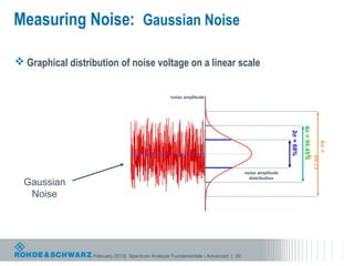
Amplitude
Noise on log (dB) scale Rayleigh Distribution
February 2013| Spectrum Analyzer Fundamentals - Advanced | 27](https://image.slidesharecdn.com/spectrumanalyzerfundamentals-advancedtruck-130221123113-phpapp02/85/Spectrum-Analyzer-Fundamentals-Advanced-Spectrum-Analysis-27-320.jpg)
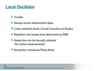
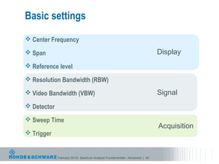
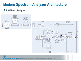
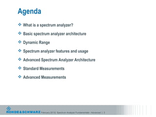
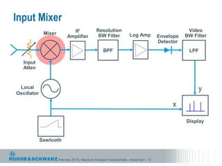
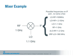
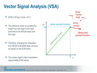
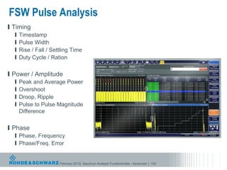
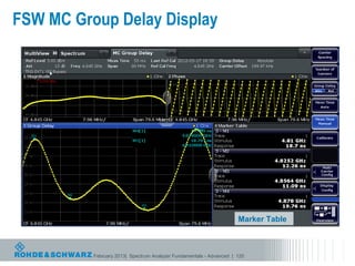
![Phase Noise
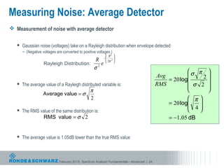
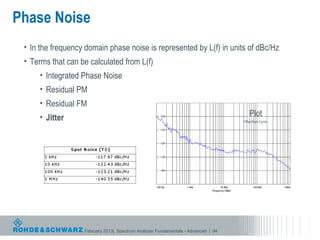
• Radom (short term) fluctuation in the phase of a waveform
Level
• Ideal Signal (noiseless)
V(t) = A sin(2πνt)
f
where
A = nominal amplitude t
ν = nominal frequency
• Real Signal Level
V(t) = [A + E(t)] sin(2πνt + φ(t))
f
where
E(t) = amplitude fluctuations t
φ(t) = phase fluctuations
Phase Noise is unintentional phase modulation on a carrier
February 2013| Spectrum Analyzer Fundamentals - Advanced | 93](https://image.slidesharecdn.com/spectrumanalyzerfundamentals-advancedtruck-130221123113-phpapp02/85/Spectrum-Analyzer-Fundamentals-Advanced-Spectrum-Analysis-92-320.jpg)


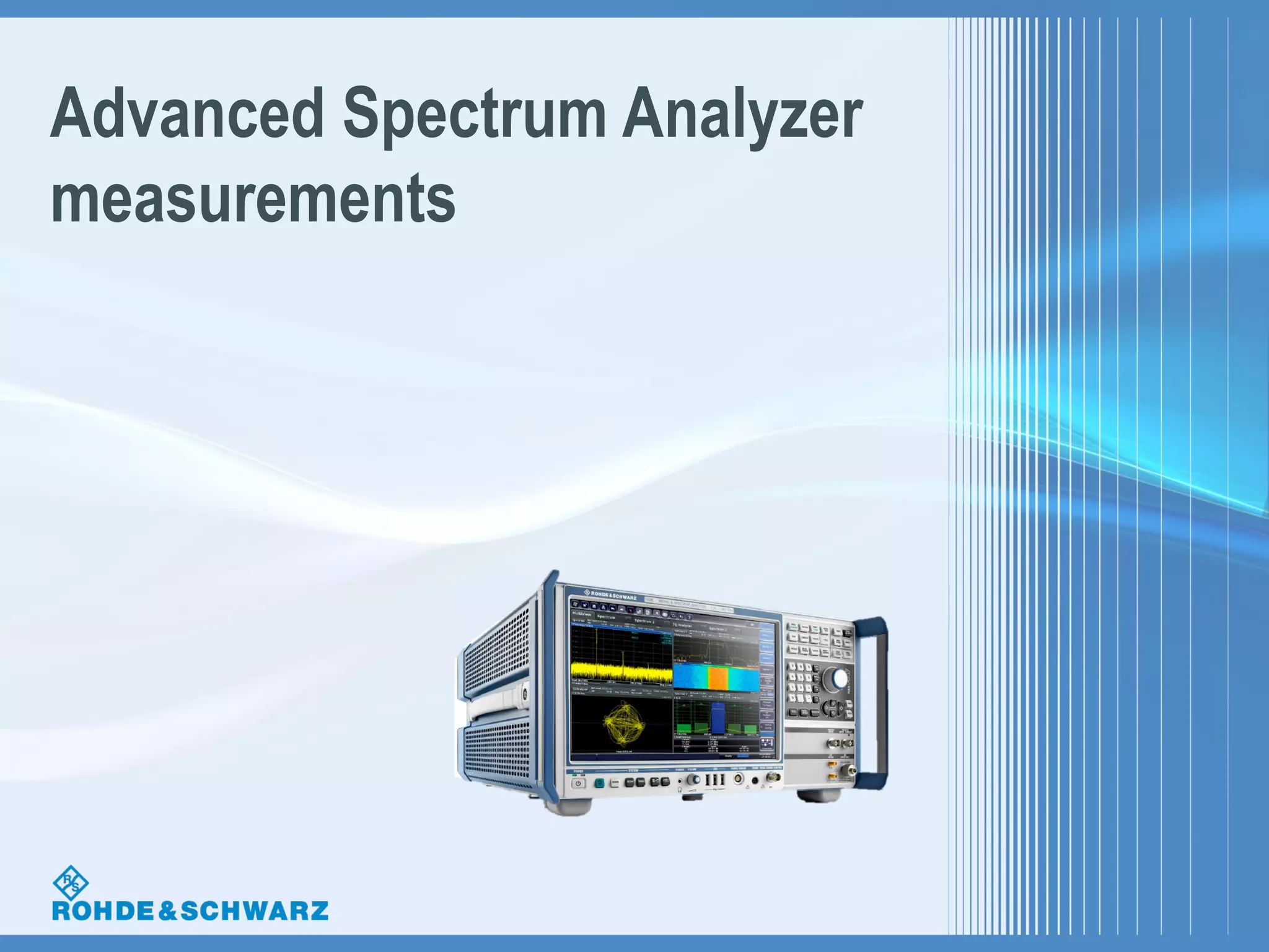
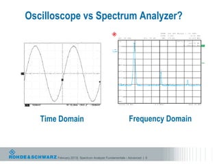
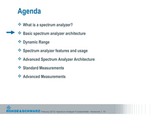
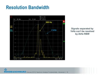
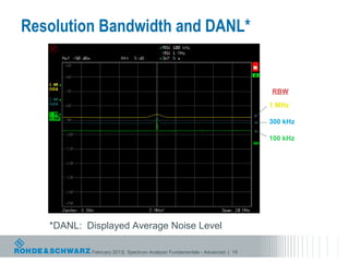
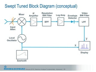
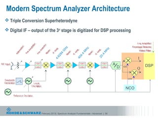
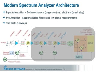
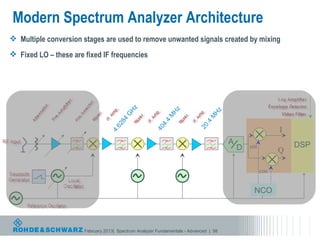
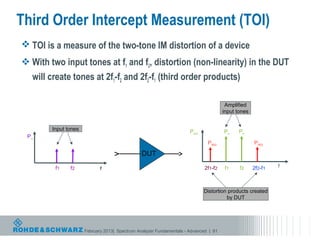
The document provides an overview of advanced spectrum analyzer measurements and architecture. It begins with a definition of a spectrum analyzer and its basic components. It then discusses features such as resolution bandwidth, detectors, and measurements over time. The document outlines the evolution of spectrum analyzer capabilities from the 1990s to present. It concludes with descriptions of standard measurements and an introduction to advanced measurements capabilities of modern spectrum analyzers.


![RF Circuit Design - [Ch4-2] LNA, PA, and Broadband Amplifier](https://cdn.slidesharecdn.com/ss_thumbnails/ch4-2-150613064410-lva1-app6891-thumbnail.jpg?width=640&height=640&fit=bounds)


![Mathematics of nyquist plot [autosaved] [autosaved]](https://cdn.slidesharecdn.com/ss_thumbnails/mathematicsofnyquistplotautosavedautosaved-150219123133-conversion-gate02-thumbnail.jpg?width=640&height=640&fit=bounds)