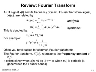
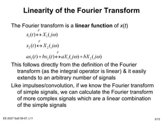
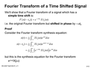
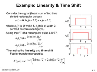
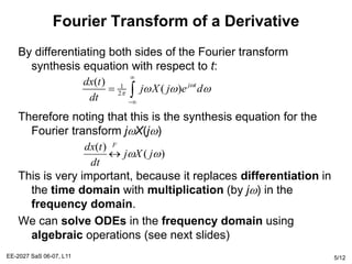
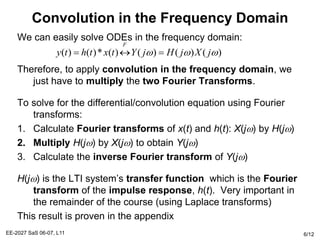
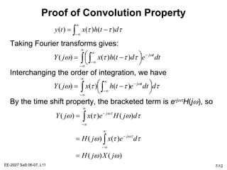
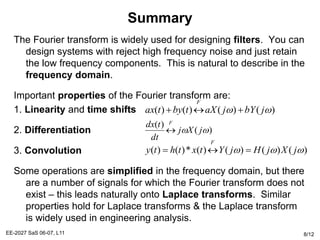
The Fourier transform relates a signal in the time domain, x(t), to its frequency domain representation, X(jw). It represents the frequency content of the signal. The Fourier transform is a linear operation, and time shifts in the time domain result in phase shifts in the frequency domain. Differentiation in the time domain corresponds to multiplication by jw in the frequency domain. Convolution becomes simple multiplication in the frequency domain. These properties allow differential equations and systems with convolution to be solved using algebraic operations by working in the frequency domain.

1. EE-2027 SaS 06-07, L11 1/12
Review: Fourier Transform
A CT signal x(t) and its frequency domain, Fourier transform signal,
X(jw), are related by
This is denoted by:
For example:
Often you have tables for common Fourier transforms
The Fourier transform, X(jw), represents the frequency content of
x(t).
It exists either when x(t)->0 as |t|->∞ or when x(t) is periodic (it
generalizes the Fourier series)









ww
w
w

w
dejXtx
dtetxjX
tj
tj
)()(
)()(
2
1
)()( wjXtx
F

wja
tue
F
at

 1
)(
analysis
synthesis

2. EE-2027 SaS 06-07, L11 2/12
Linearity of the Fourier Transform
The Fourier transform is a linear function of x(t)
This follows directly from the definition of the Fourier
transform (as the integral operator is linear) & it easily
extends to an arbitrary number of signals
Like impulses/convolution, if we know the Fourier transform
of simple signals, we can calculate the Fourier transform
of more complex signals which are a linear combination
of the simple signals
1 1
2 2
1 2 1 2
( ) ( )
( ) ( )
( ) ( ) ( ) ( )
F
F
F
x t X j
x t X j
ax t bx t aX j bX j
w
w
w w


  

3. EE-2027 SaS 06-07, L11 3/12
Fourier Transform of a Time Shifted Signal
We’ll show that a Fourier transform of a signal which has a
simple time shift is:
i.e. the original Fourier transform but shifted in phase by –wt0
Proof
Consider the Fourier transform synthesis equation:
but this is the synthesis equation for the Fourier transform
e-jw0tX(jw)
 
0
0
1
2
( )1
0 2
1
2
( ) ( )
( ) ( )
( )
j t
j t t
j t j t
x t X j e d
x t t X j e d
e X j e d
w

w

w w

w w
w w
w w









 




)()}({ 0
0 ww
jXettxF tj


4. EE-2027 SaS 06-07, L11 4/12
Example: Linearity & Time Shift
Consider the signal (linear sum of two time
shifted rectangular pulses)
where x1(t) is of width 1, x2(t) is of width 3,
centred on zero (see figures)
Using the FT of a rectangular pulse L10S7
Then using the linearity and time shift
Fourier transform properties
)5.2()5.2(5.0)( 21  txtxtx
w
ww )2/sin(2)(1 jX
  



  
w
www w )2/3sin(2)2/sin()( 2/5j
ejX
w
ww )2/3sin(2)(2 jX
t
t
t
x1(t)
x2(t)
x (t)

5. EE-2027 SaS 06-07, L11 5/12
Fourier Transform of a Derivative
By differentiating both sides of the Fourier transform
synthesis equation with respect to t:
Therefore noting that this is the synthesis equation for the
Fourier transform jwX(jw)
This is very important, because it replaces differentiation in
the time domain with multiplication (by jw) in the
frequency domain.
We can solve ODEs in the frequency domain using
algebraic operations (see next slides)
)(
)(
ww jXj
dt
tdx F

1
2
( )
( ) j tdx t
j X j e d
dt
w
 w w w


 

6. EE-2027 SaS 06-07, L11 6/12
Convolution in the Frequency Domain
We can easily solve ODEs in the frequency domain:
Therefore, to apply convolution in the frequency domain, we
just have to multiply the two Fourier Transforms.
To solve for the differential/convolution equation using Fourier
transforms:
1. Calculate Fourier transforms of x(t) and h(t): X(jw) by H(jw)
2. Multiply H(jw) by X(jw) to obtain Y(jw)
3. Calculate the inverse Fourier transform of Y(jw)
H(jw) is the LTI system’s transfer function which is the Fourier
transform of the impulse response, h(t). Very important in
the remainder of the course (using Laplace transforms)
This result is proven in the appendix
)()()()(*)()( www jXjHjYtxthty
F


7. EE-2027 SaS 06-07, L11 7/12
Proof of Convolution Property
Taking Fourier transforms gives:
Interchanging the order of integration, we have
By the time shift property, the bracketed term is e-jwtH(jw), so



 ttt dthxty )()()(
 









  dtedthxjY tjw
tttw )()()(
 









  tttw w
ddtethxjY tj
)()()(
)()(
)()(
)()()(
ww
ttw
twtw
wt
wt
jXjH
dexjH
djHexjY
j
j












8. EE-2027 SaS 06-07, L11 8/12
Summary
The Fourier transform is widely used for designing filters. You can
design systems with reject high frequency noise and just retain
the low frequency components. This is natural to describe in the
frequency domain.
Important properties of the Fourier transform are:
1. Linearity and time shifts
2. Differentiation
3. Convolution
Some operations are simplified in the frequency domain, but there
are a number of signals for which the Fourier transform does not
exist – this leads naturally onto Laplace transforms. Similar
properties hold for Laplace transforms & the Laplace transform
is widely used in engineering analysis.
)(
)(
ww jXj
dt
tdx F

)()()()(*)()( www jXjHjYtxthty
F

)()()()( ww jbYjaXtbytax
F
