Lesson05_Static11

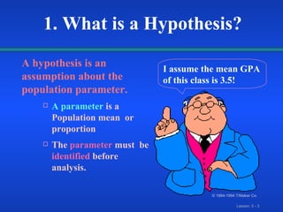
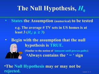
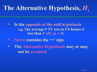
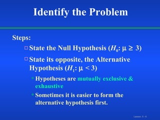
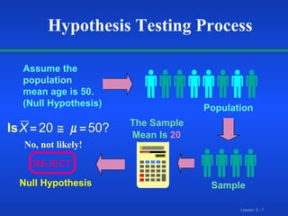
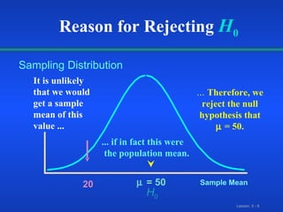
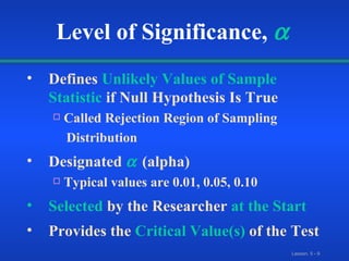
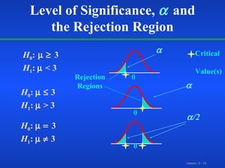
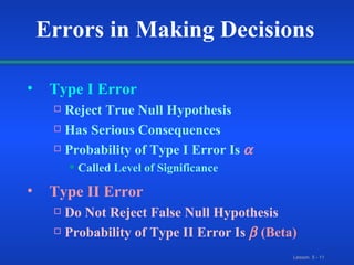
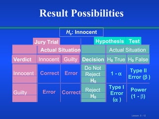
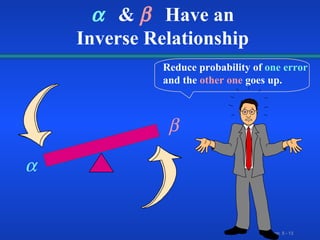
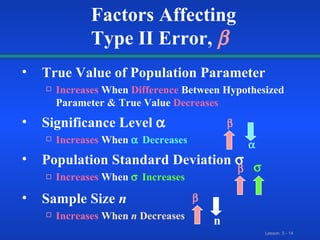
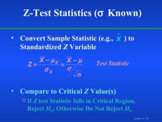
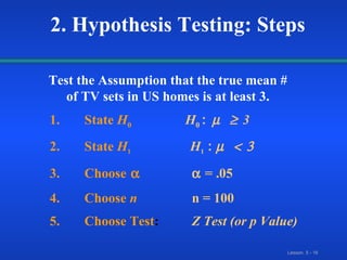
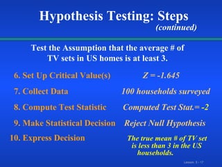
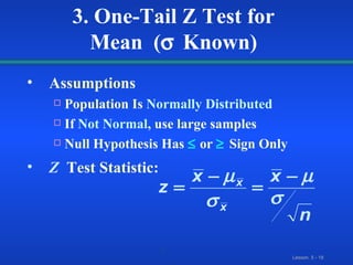
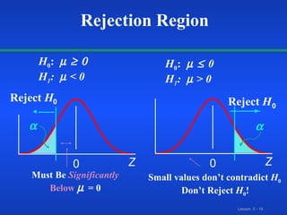
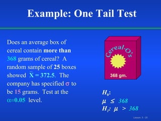
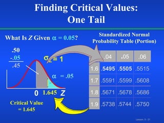
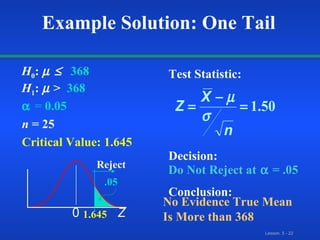
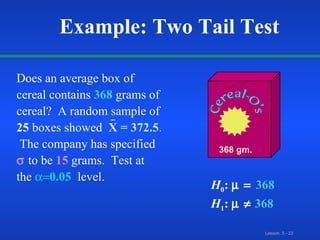
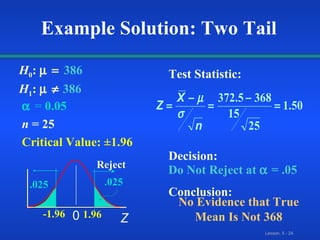
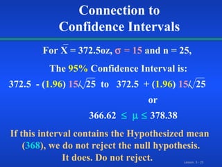
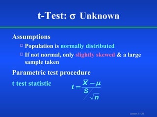
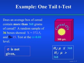
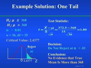
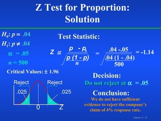
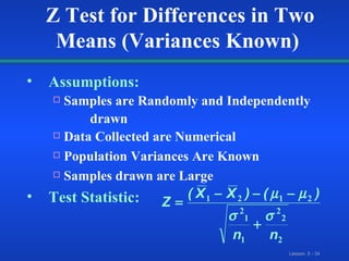
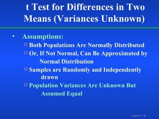
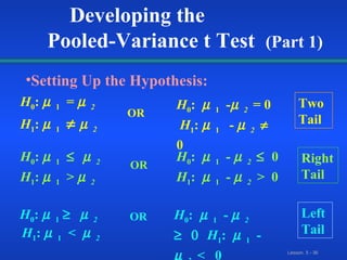
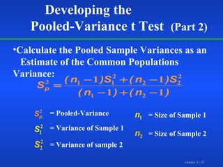
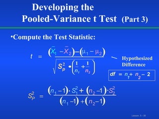
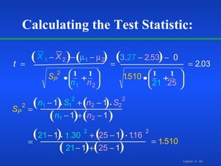
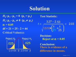
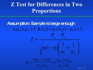
Statistics for Management Fundamentals of Hypothesis Testing

Lesson Topics 1. What is a Hypothesis? Hypothesis Testing Methodology Hypothesis Testing Process Level of Significance, a Errors in Making Decisions 2. Hypothesis Testing: Steps Z Test for the Mean (s Known) Connection to Confidence Interval Estimation Hypothesis Testing Methodology

[object Object],[object Object],[object Object],[object Object],The Null Hypothesis, H 0 ,[object Object],[object Object]

[object Object],[object Object],[object Object],The Alternative Hypothesis, H 1

[object Object],[object Object],[object Object],[object Object],[object Object],Identify the Problem

Population Assume the population mean age is 50. (Null Hypothesis) REJECT The Sample Mean Is 20 Sample Null Hypothesis Hypothesis Testing Process No, not likely!

Sample Mean  = 50 Sampling Distribution It is unlikely that we would get a sample mean of this value ... ... if in fact this were the population mean. ... Therefore, we reject the null hypothesis that  = 50. 20 H 0 Reason for Rejecting H 0

[object Object],[object Object],[object Object],[object Object],[object Object],[object Object],[object Object],Level of Significance, 

Level of Significance,  and the Rejection Region H 0 :   3 H 1 :  < 3 0 0 0 H 0 :   3 H 1 :  > 3 H 0 :   3 H 1 :   3    /2 Critical Value(s) Rejection Regions

[object Object],[object Object],[object Object],[object Object],[object Object],[object Object],[object Object],[object Object],Errors in Making Decisions

H 0 : Innocent Jury Trial Hypothesis Test Actual Situation Actual Situation Verdict Innocent Guilty Decision H 0 True H 0 False Innocent Correct Error Do Not Reject H 0 1 -  Type II Error (  ) Guilty Error Correct Reject H 0 Type I Error (  ) Power (1 -  ) Result Possibilities

  Reduce probability of one error and the other one goes up.  &   Have an Inverse Relationship

[object Object],[object Object],[object Object],[object Object],[object Object],[object Object],[object Object],[object Object],Factors Affecting Type II Error,       n

[object Object],[object Object],[object Object],Z-Test Statistics (  Known) Test Statistic X

[object Object],[object Object],[object Object],[object Object],[object Object],2. Hypothesis Testing: Steps Test the Assumption that the true mean # of TV sets in US homes is at least 3.

[object Object],[object Object],[object Object],[object Object],[object Object],Hypothesis Testing: Steps Test the Assumption that the average # of TV sets in US homes is at least 3. (continued)

[object Object],[object Object],[object Object],[object Object],[object Object],3. One-Tail Z Test for Mean (  Known)

Z 0  Reject H 0 Z 0 Reject H 0  H 0 :  H 1 :  < 0 H 0 :  0 H 1 :  > 0 Must Be Significantly Below  = 0 Small values don’t contradict H 0 Don’t Reject H 0 ! Rejection Region

[object Object],368 gm. Example: One Tail Test H 0 :  368 H 1 :  > 368 _

Z .04 .06 1.6 . 5495 . 5505 .5515 1.7 .5591 .5599 .5608 1.8 .5671 .5678 .5686 .5738 .5750 Z 0  Z = 1 1.645 .50 -. 05 .45 . 05 1.9 .5744 Standardized Normal Probability Table (Portion) What Is Z Given   = 0.05 ?  = .05 Finding Critical Values: One Tail Critical Value = 1.645

[object Object],[object Object],[object Object],Test Statistic: Decision: Conclusion: Do Not Reject at  = .05 No Evidence True Mean Is More than 368 Z 0 1.645 .05 Reject Example Solution: One Tail H 0 :  368 H 1 :  > 368

[object Object],368 gm. Example: Two Tail Test H 0 :  368 H 1 :  368

[object Object],[object Object],[object Object],Test Statistic: Decision: Conclusion: Do Not Reject at  = .05 No Evidence that True Mean Is Not 368 Z 0 1.96 .025 Reject Example Solution: Two Tail -1.96 .025 H 0 :  386 H 1 :  386

Connection to Confidence Intervals ,[object Object],[object Object],[object Object],[object Object],[object Object],[object Object],[object Object],_

[object Object],[object Object],[object Object],[object Object],[object Object],t-Test:  Unknown

Example: One Tail t-Test Does an average box of cereal contain more than 368 grams of cereal? A random sample of 36 boxes showed X = 372.5 , and  S= 15 . Test at the  0.01 level. 368 gm. H 0 :   368 H 1 :  368  is not given,

[object Object],[object Object],[object Object],Test Statistic: Decision: Conclusion: Do Not Reject at  = .01 No Evidence that True Mean Is More than 368 Z 0 2.4377 .01 Reject Example Solution: One Tail H 0 :  368 H 1 :  368

[object Object],[object Object],[object Object],[object Object],[object Object],[object Object],4. Proportions

Example:Z Test for Proportion ,[object Object],[object Object],[object Object]

[object Object],[object Object],Do not reject at  = .05 Z Test for Proportion: Solution H 0 : p  .04 H 1 : p  .04 Critical Values:  1.96 Test Statistic: Decision: Conclusion: We do not have sufficient evidence to reject the company’s claim of 4% response rate. Z  p - p p (1 - p) n s = .04 -.05 .04 (1 - .04) 500 = -1.14 Z 0 Reject Reject .025 .025

5. Comparing two independent samples ,[object Object],[object Object],[object Object],[object Object],[object Object],[object Object],[object Object]

[object Object],[object Object],[object Object],[object Object],[object Object],[object Object],[object Object],Independent Samples

[object Object],[object Object],[object Object],[object Object],[object Object],[object Object],[object Object],Z Test for Differences in Two Means (Variances Known)

[object Object],[object Object],[object Object],[object Object],[object Object],[object Object],[object Object],[object Object],t Test for Differences in Two Means (Variances Unknown)

Developing the Pooled-Variance t Test (Part 1) ,[object Object],H 0 :  1   2 H 1 :  1 >  2 H 0 :  1 -  2 = 0 H 1 :  1 -  2  0 H 0 :  1 =  2 H 1 :  1   2 H 0 :  1   2  H 0 :  1 -  2  0 H 1 :  1 -  2 > 0 H 0 :  1 -  2  H 1 :  1 -  2 < 0 OR OR OR Left Tail Right Tail Two Tail  H 1 :  1 <  2

Developing the Pooled-Variance t Test (Part 2) ,[object Object],= Pooled-Variance = Variance of Sample 1 = Variance of sample 2 = Size of Sample 1 = Size of Sample 2

t X X S n S n S n n df n n P                 1 2 1 2 2 1 1 2 2 2 2 1 2 1 2 1 1 1 1 2   Hypothesized Difference Developing the Pooled-Variance t Test (Part 3) ,[object Object],( ) ) ( ( ) ( ) ( ) ( ) n 1 n 2 _ _

t X X S n n S n S n S n n P P                            1 2 1 2 2 1 2 2 1 1 2 2 2 2 1 2 2 2 3 27 2 53 0 1 510 21 25 2 03 1 1 1 1 21 1 1 30 25 1 1 16 21 1 25 1 1 510   . . . . . . . Calculating the Test Statistic: ( ( ( ( ( ( ( ( ( ( ( ) ) ) ) ) ) ) ) ) ) )

[object Object],[object Object],[object Object],[object Object],[object Object],Test Statistic: Decision: Conclusion: Reject at  = 0.05 There is evidence of a difference in means. t 0 2.0154 -2.0154 .025 Reject H 0 Reject H 0 .025 t    3 27 2 53 1 510 21 25 2 03 . . . . Solution

Z Test for Differences in Two Proportions ,[object Object]

Lesson05_Static11

Recommended

Recommended

More Related Content

What's hot

What's hot (18)

Similar to Lesson05_Static11

Similar to Lesson05_Static11 (20)

More from thangv

More from thangv (17)

Recently uploaded

Recently uploaded (20)

Lesson05_Static11