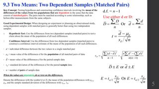
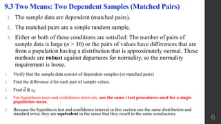
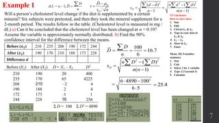
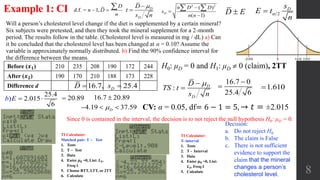
This document discusses testing differences between two dependent samples using matched pairs. It provides examples of how to: 1) Calculate the differences between matched pairs and find the mean and standard deviation of the differences. 2) Use a t-test to determine if the mean difference is statistically significant and construct a 90% confidence interval for the true mean difference between two dependent samples. 3) Apply these methods to an example comparing cholesterol levels before and after a mineral supplement, testing the claim that the supplement changes cholesterol levels.

1. Elementary Statistics
Chapter 9:
Inferences from Two
Samples
9.3 Two Dependent
Samples (Matched
Pairs)
1

2. Chapter 9: Inferences from Two Samples
9. 1 Two Proportions
9.2 Two Means: Independent Samples
9.3 Two Dependent Samples (Matched Pairs)
9.4 Two Variances or Standard Deviations
2
Objectives:
• Test the difference between two proportions.
• Test the difference between sample means, using the z test.
• Test the difference between two means for independent samples, using the t test.
• Test the difference between two means for dependent samples.
• Test the difference between two variances or standard deviations.

3. For population 1 & 2:
Recall: Chapter 9.1: Inferences about Two Proportions
1 2
1 2
X X
p
n n



1q p 
The pooled sample proportion combines the two samples
proportions into one proportion & Test Statistic :
       1 2 1 2 1 2 1 2
1 21 2
ˆ ˆ ˆ ˆ
: Or
1 1
p p p p p p p p
TS z
pq pq
pq
n nn n
     

   
 
Confidence Interval Estimate of p1 − p2
   1 1 2 2 1 1 2 2
1 2 2 1 2 1 2 2
1 2 1 2
ˆ ˆ ˆ ˆ ˆ ˆ ˆ ˆ
ˆ ˆ ˆ ˆ
p q p q p q p q
p p z p p p p z
n n n n
         
 1 2
ˆ ˆp p E 
The P-value method and the critical value method are equivalent, but the confidence
interval method is not equivalent to the P-value method or the critical value method.
2
2 2 2
2
ˆ ˆ ˆ, 1
x
p q p
n
  1
1 1 1
1
ˆ ˆ ˆ, 1
x
p q p
n
  
3
TI Calculator:
Confidence Interval: 2
proportion
1. Stat
2. Tests
3. 2-prop ZINT
4. Enter:𝒏 𝟏 , 𝒏 𝟐, 𝒙 𝟏, 𝒙 𝟐 & CL
TI Calculator:
2 - Proportion Z - test
1. Stat
2. Tests
3. 2 ‒ PropZTest
4. Enter Data or Stats
𝒏 𝟏 , 𝒏 𝟐, 𝒙 𝟏, 𝒙 𝟐
5. Choose RTT, LTT,
or 2TT

4. Recall: 9.2 Two Means: Independent Samples: 1. The two samples are
independent. 2. Both samples are simple random samples. 3. Either or both of
these conditions are satisfied: The two sample sizes are both large (with n1 > 30 and n2
> 30) or both samples come from populations having normal distributions.
σ1 and σ2 are known: Use the z test for comparing two means from independent populations
2 2
1 2
2
1 2
E z
n n

 
 1 2
Confidence Inte
)
rv
(
al:
x x E 
1 2 1 2 1 2
2 2 2 2
1 2 1 2
1 2 1 2
( ) ( )
: Or
x x x x
TS z z
n n n n
 
   
   
 
 
2 2
1 2
2
1 2
s s
E t
n n
 
Unequal Variances: σ1 ≠ σ2
df = smaller of n1 – 1 or n2 – 1
Equal Variances :
σ1 = σ2
Pool the Sample
Variances
df = n1 – 1 + n2 – 1
1 2
2 2
1 2
1 2
:
x x
TS t
s s
n n



1 2
2 2
1 2
:
p p
x x
TS t
s s
n n



σ1 and σ2 are unknown: Use the t test for comparing two means from independent populations
2 2
1 1 2 2
1 2
( 1) ( 1)
( 1) ( 1)
p
n s n s
s
n n
  

  
2 2
2
1 2
p ps s
E t
n n
 
4
TI Calculator:
2 - Sample Z - test
1. Stat
2. Tests
3. 2 ‒ SampZTest
4. Enter Data or Stats
𝝈 𝟏 , 𝝈 𝟐, 𝒙 𝟏 , 𝒏 𝟏, 𝒙 𝟐
𝒏 𝟏 , 𝒏 𝟐,
5. Choose RTT, LTT,
or 2TT
6. Calculate
TI Calculator:
2 - Sample Z - Interval
1. Stat
2. Tests
3. 2 ‒ SampZInt
4. Enter Data or Stats
𝝈 𝟏 , 𝝈 𝟐, 𝒙 𝟏 , 𝒏 𝟏, 𝒙 𝟐
𝒏 𝟏 , 𝒏 𝟐,
5. Choose RTT, LTT, or
2TT
6. Calculate
TI Calculator:
2 - Sample T - test
1. Stat
2. Tests
3. 2 ‒ SampTTest
4. Enter Data or Stats
𝒙 𝟏, 𝒔 𝟏 , 𝒏 𝟏, 𝒙 𝟐
𝒏 𝟏 , 𝒔 𝟐,
5. Choose RTT, LTT,
or 2TT
6. Pooled: No / Yes
7. Calculate
TI Calculator:
2 - Sample T - Interval
1. Stat
2. Tests
3. 2 ‒ SampTInt
4. Enter Data or Stats
𝒙 𝟏, 𝒔 𝟏 , 𝒏 𝟏, 𝒙 𝟐
𝒏 𝟏 , 𝒔 𝟐,
5. Choose RTT, LTT,
or 2TT
6. Pooled: No / Yes
7. Calculate

5. Key Concept: Testing hypotheses and constructing confidence intervals involving the mean of the
differences of the values from two populations that are dependent in the sense that the data
consist of matched pairs. The pairs must be matched according to some relationship, such as
before/after measurements from the same subjects .
Good Experimental Design: When designing an experiment or planning an observational study,
using dependent samples with matched pairs is generally better than using two independent
samples.
1. Hypothesis Test: Use the differences from two dependent samples (matched pairs) to test a
claim about the mean of the population of all such differences.
2. Confidence Interval: Use the differences from two dependent samples (matched pairs) to
construct a confidence interval estimate of the mean of the population of all such differences.
• d = individual difference between the two values in a single matched pair
• µd = mean value of the differences d for the population of all matched pairs of data
• 𝑑 = mean value of the differences d for the paired sample data
• sd = standard deviation of the differences d for the paired sample data
• n = number of pairs of sample data
When the values are dependent, do a t test on the differences.
Denote the differences with the symbol d or D, the mean of the population differences with μd or
μD, and the sample standard deviation of the differences with sd or sD.
9.3 Two Means: Two Dependent Samples (Matched Pairs)
5
Use either d or
d.f. = 1
Or
D:
n
D d
D d
n n

 
 
d
d
d
t
s n


orD E d E 
2 2OrD ds s
E t E t
n n
  
2 2 2
( ) ( )
1 ( 1)
D
d d n d d
s
n n n
 
 
 
  

6. 1. The sample data are dependent (matched pairs).
2. The matched pairs are a simple random sample.
3. Either or both of these conditions are satisfied: The number of pairs of
sample data is large (n > 30) or the pairs of values have differences that are
from a population having a distribution that is approximately normal. These
methods are robust against departures for normality, so the normality
requirement is loose.
6
9.3 Two Means: Two Dependent Samples (Matched Pairs)
1. Verify that the sample data consist of dependent samples (or matched pairs)
2. Find the difference d for each pair of sample values.
3. Find 𝑑 & 𝑠 𝑑
4. For hypothesis tests and confidence intervals, use the same t test procedures used for a single
population mean.
5. Because the hypothesis test and confidence interval in this section use the same distribution and
standard error, they are equivalent in the sense that they result in the same conclusions.

7. 7
Will a person’s cholesterol level change if the diet is supplemented by a certain
mineral? Six subjects were pretested, and then they took the mineral supplement for a
2-month period. The results follow in the table. (Cholesterol level is measured in mg /
dL) a) Can it be concluded that the cholesterol level has been changed at α = 0.10?
Assume the variable is approximately normally distributed. b) Find the 90%
confidence interval for the difference between the means.
Example 1
Before (𝒙 𝟏) 210 235 208 190 172 244
After (𝒙 𝟐) 190 170 210 188 173 228
Difference d
d.f. = 1,
D
n D
n
 
 
 D
D
D
t
s n

Before (X1) After (X2) D = X1 – X2 D2
210
235
208
190
172
244
190
170
210
188
173
228
20
65
–2
2
–1
16
400
4225
4
4
1
256
Σ D = 100 Σ D2 = 4890
100
16.7
6
  
D
D
n
2 2
( )
( 1)
D
n D D
s
n n



 
2
6 4890 100
6 5
 


25.4
2 2 2
( ) ( )
1 ( 1)
D
d d n d d
s
n n n
 
 
 
  
TI Calculator:
How to enter data:
1. Stat
2. Edit
3. ClrList 𝑳 𝟏 & 𝑳 𝟐
4. Type in your data in
𝑳 𝟏 & 𝑳 𝟐
5. 𝑳 𝟏 − 𝑳 𝟐
6. Store in 𝑳 𝟑
7. Enter
Mean, SD, 5-number
summary
1. Stat
2. Calc
3. Select 1 for 1 variable
4. Type: L3 (second 3)
5. Calculate

8. 8
Will a person’s cholesterol level change if the diet is supplemented by a certain mineral?
Six subjects were pretested, and then they took the mineral supplement for a 2-month
period. The results follow in the table. (Cholesterol level is measured in mg / dL) a) Can
it be concluded that the cholesterol level has been changed at α = 0.10? Assume the
variable is approximately normally distributed. b) Find the 90% confidence interval for
the difference between the means.
Example 1: CI
CV: α = 0.05, df= 6 − 1 = 5, → 𝑡 = ±2.015
H0: μD = 0 and H1: μD  0 (claim), 2TTBefore (𝒙 𝟏) 210 235 208 190 172 244
After (𝒙 𝟐) 190 170 210 188 173 228
Difference d
d.f. = 1,
D
n D
n
 
 
 D
D
D
t
s n

16.7, 25.4 DD s : D
D
D
TS t
s n


16.7 0
25.4 6

 1.610
Decision:
a. Do not reject H0
b. The claim is False
c. There is not sufficient
evidence to support the
claim that the mineral
changes a person’s
cholesterol level.
25.4
2.015
6
)b E   16.7 20.89
4.19 37.59  D
20.89
D E 2
Ds
E t
n

Since 0 is contained in the interval, the decision is to not reject the null hypothesis H0: μD = 0.
2 2
( )
( 1)
D
n D D
s
n n



 
TI Calculator:
T- interval
1. Tests
2. T - Interval
3. Data
4. Enter 𝝁 𝟎 =0, List:
𝑳 𝟑, Freq:1
5. Calculate
TI Calculator:
Matched pair: T ‒ Test
1. Tests
2. T ‒ Test
3. Data
4. Enter 𝝁 𝟎 =0, List: 𝑳 𝟑,
Freq:1
5. Choose RTT, LTT, or 2TT
6. Calculate