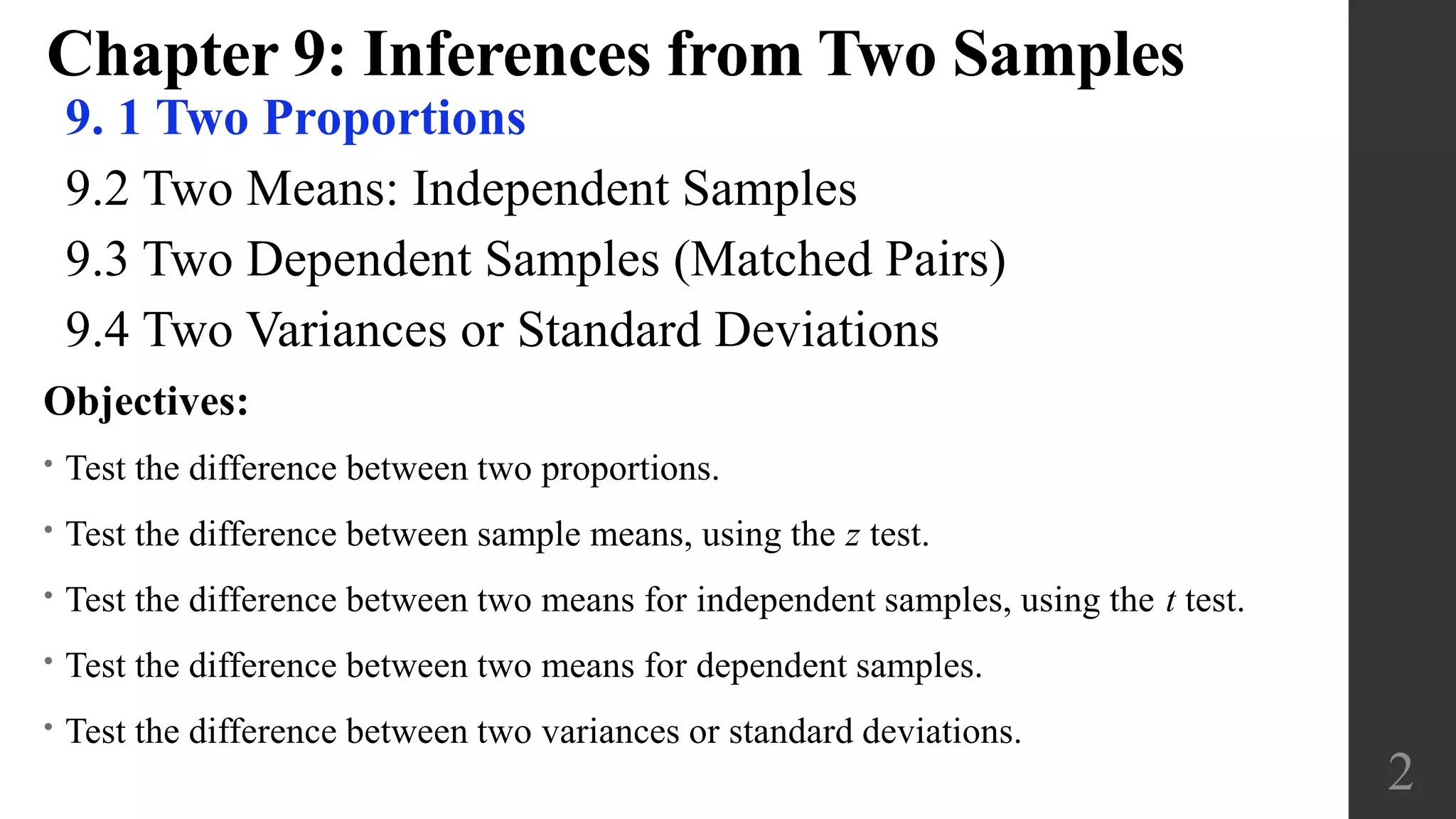
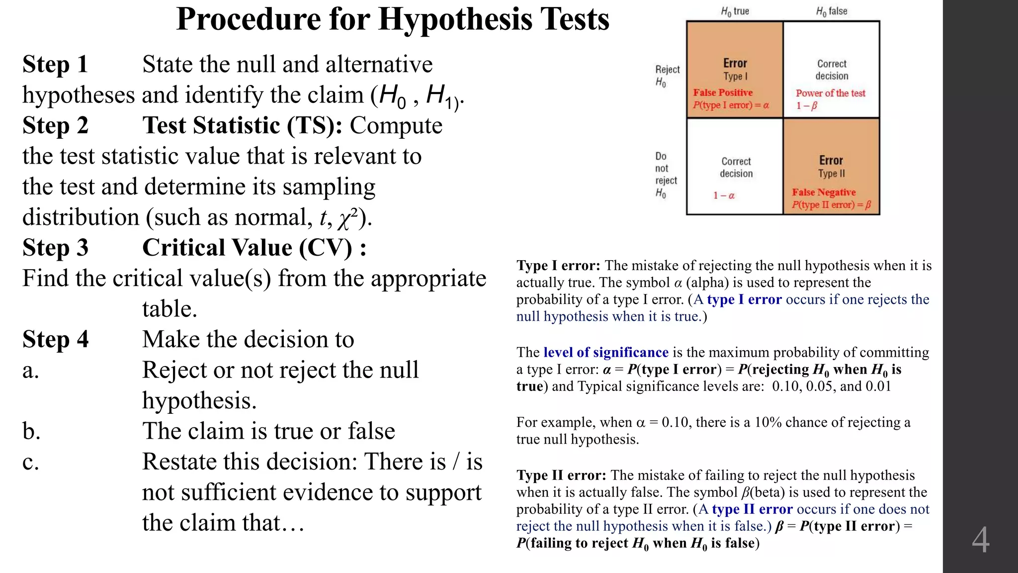
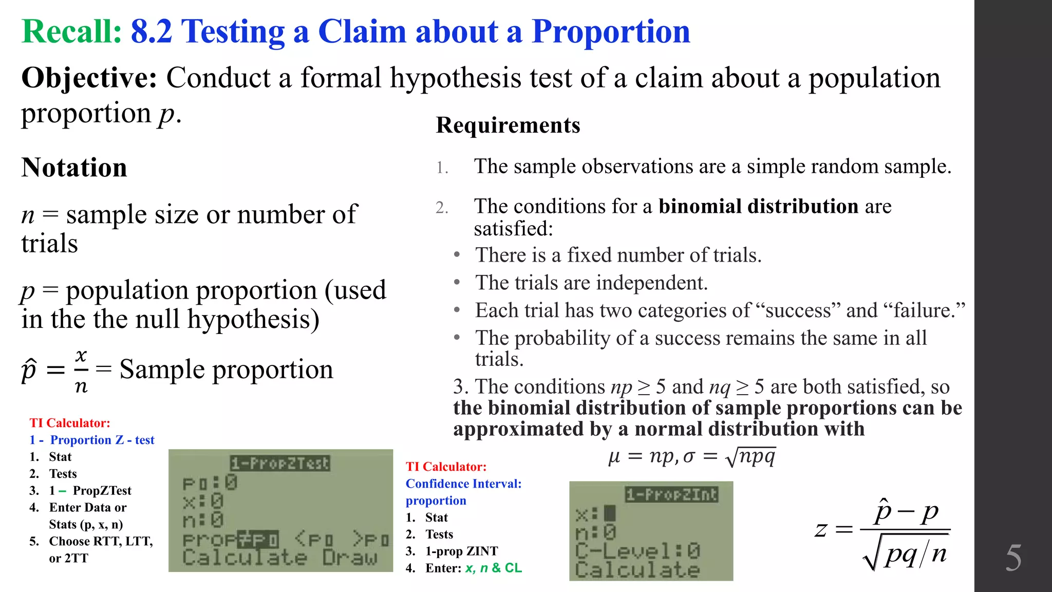
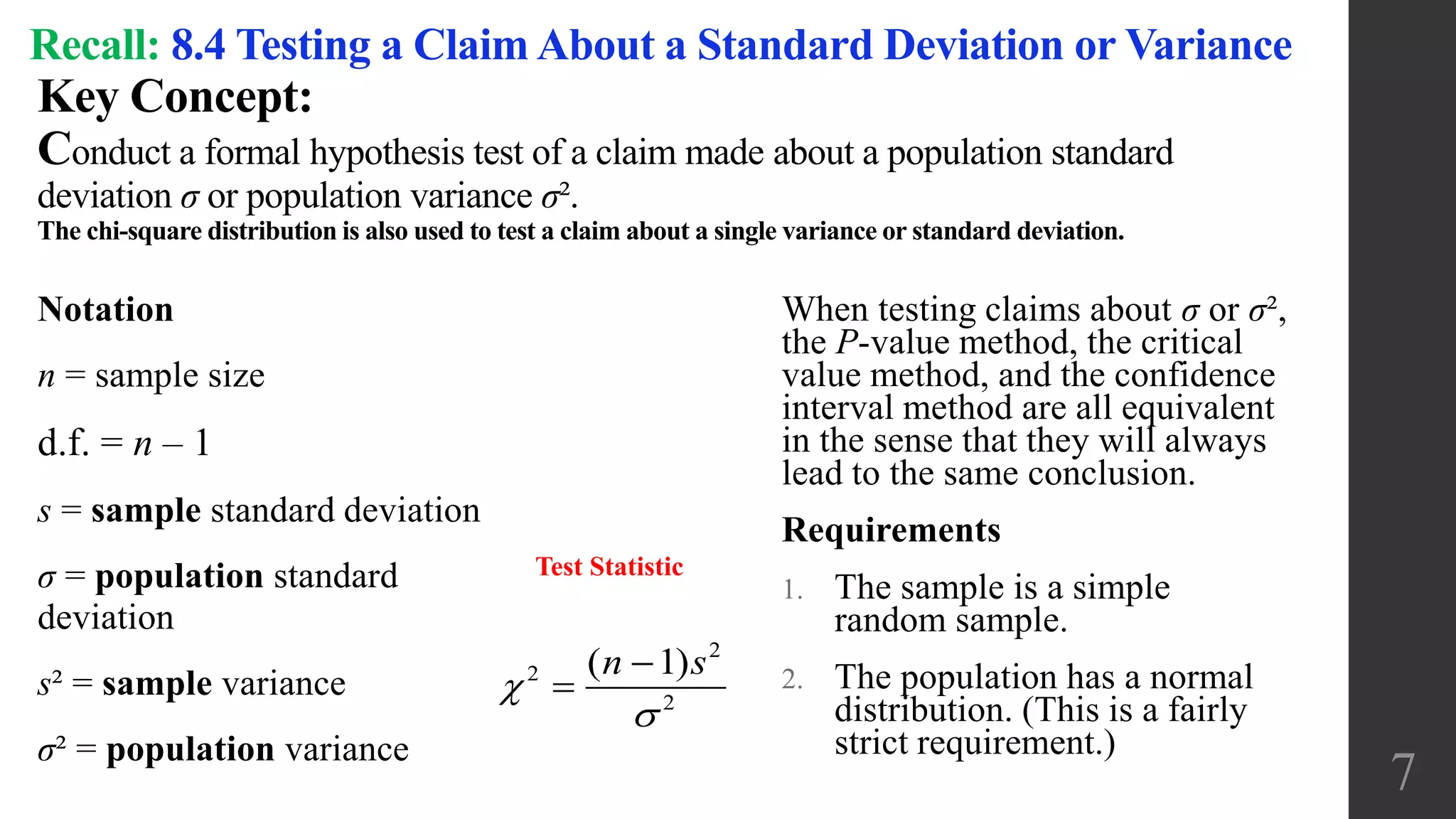
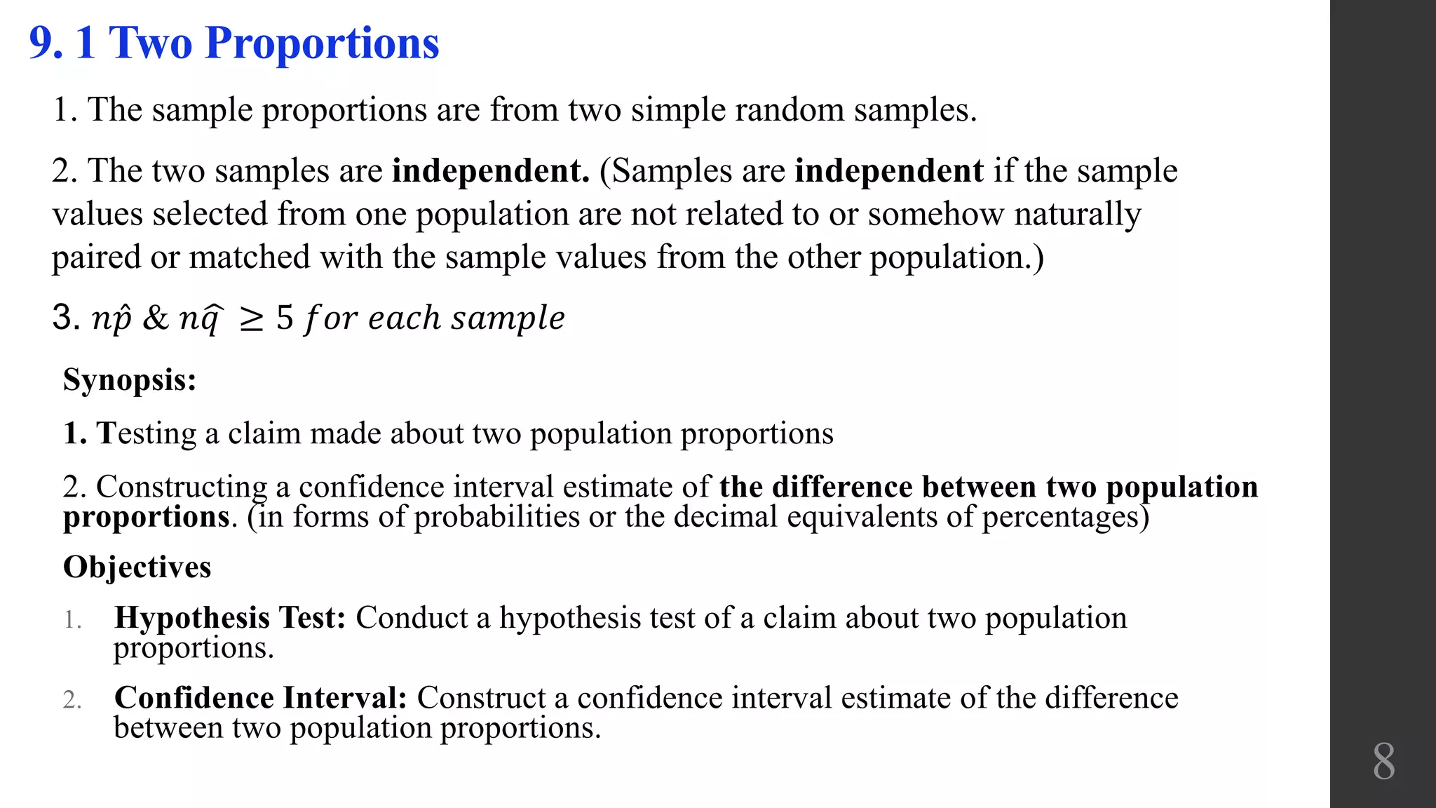
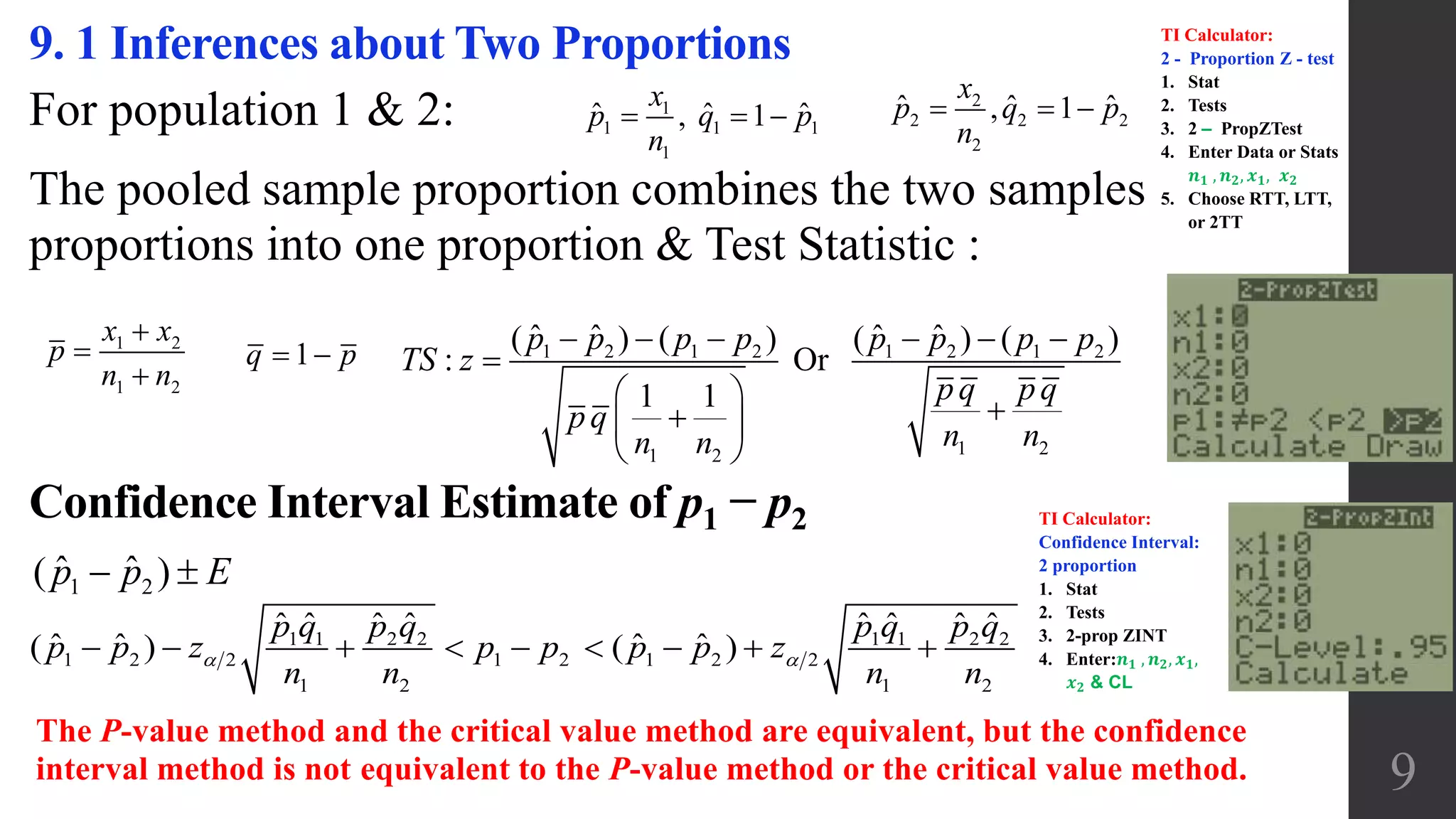
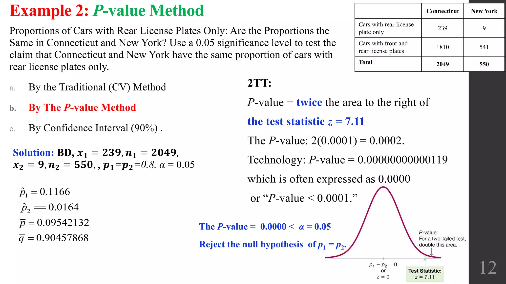
Elementary Statistics
Chapter 9:
Inferences from Two
Samples
9. 1 Two Proportions
1
Chapter 9: Inferences from Two Samples
9. 1 Two Proportions
9.2 Two Means: Independent Samples
9.3 Two Dependent Samples (Matched Pairs)
9.4 Two Variances or Standard Deviations
2
Objectives:
• Test the difference between two proportions.
• Test the difference between sample means, using the z test.
• Test the difference between two means for independent samples, using the t test.
• Test the difference between two means for dependent samples.
• Test the difference between two variances or standard deviations.
1. The traditional method (Critical Value Method) (CV)
2. The P-value method
P-Value Method: In a hypothesis test, the P-value is the probability of getting a value of the
test statistic that is at least as extreme as the test statistic obtained from the sample data,
assuming that the null hypothesis is true.
3. The confidence interval (CI)method
Because a confidence interval estimate of a population parameter contains the likely values of that parameter,
reject a claim that the population parameter has a value that is not included in the confidence interval.
Equivalent Methods: A confidence interval estimate of a proportion might lead to a conclusion different
from that of a hypothesis test.
Recall: 8.1 Basics of Hypothesis Testing: 3 methods used to test hypotheses:
3
Construct a confidence interval with
a confidence level selected:
Significance Level for
Hypothesis Test: α
Two-Tailed Test:
1 – α
One-Tailed
Test: 1 – 2α
0.01 99% 98%
0.05 95% 90%
0.10 90% 80%
A statistical hypothesis is a assumption about a population parameter. This conjecture may or may not be
true. The null hypothesis, symbolized by H0, and the alternative hypothesis, symbolized by H1
4
Type I error: The mistake of rejecting the null hypothesis when it is
actually true. The symbol α (alpha) is used to represent the
probability of a type I error. (A type I error occurs if one rejects the
null hypothesis when it is true.)
The level of significance is the maximum probability of committing
a type I error: α = P(type I error) = P(rejecting H0 when H0 is
true) and Typical significance levels are: 0.10, 0.05, and 0.01
For example, when a = 0.10, there is a 10% chance of rejecting a
true null hypothesis.
Type II error: The mistake of failing to reject the null hypothesis
when it is actually false. The symbol β(beta) is used to represent the
probability of a type II error. (A type II error occurs if one does not
reject the null hypothesis when it is false.) β = P(type II error) =
P(failing to reject H0 when H0 is false)
Procedure for Hypothesis Tests
Step 1 State the null and alternative
hypotheses and identify the claim (H0 , H1).
Step 2 Test Statistic (TS): Compute
the test statistic value that is relevant to
the test and determine its sampling
distribution (such as normal, t, χ²).
Step 3 Critical Value (CV) :
Find the critical value(s) from the appropriate
table.
Step 4 Make the decision to
a. Reject or not reject the null
hypothesis.
b. The claim is true or false
c. Restate this decision: There is / is
not sufficient evidence to support
the claim that…
Objective: Conduct a formal hypothesis test of a claim about a population
proportion p.
Recall: 8.2 Testing a Claim about a Proportion
Notation
n = sample size or number of
trials
p = population proportion (used
in the the null hypothesis)
𝑝 =
𝑥
𝑛
= Sample proportion
Requirements
1. The sample observations are a simple random sample.
2. The conditions for a binomial distribution are
satisfied:
• There is a fixed number of trials.
• The trials are independent.
• Each trial has two categories of “success” and “failure.”
• The probability of a success remains the same in all
trials.
3. The conditions np ≥ 5 and nq ≥ 5 are both satisfied, so
the binomial distribution of sample proportions can be
approximated by a normal distribution with
𝜇 = 𝑛𝑝, 𝜎 = 𝑛𝑝𝑞
5
ˆ 

p p
z
pq n
TI Calculator:
1 - Proportion Z - test
1. Stat
2. Tests
3. 1 ‒ PropZTest
4. Enter Data or
Stats (p, x, n)
5. Choose RTT, LTT,
or 2TT
TI Calculator:
Confidence Interval:
proportion
1. Stat
2. Tests
3. 1-prop ZINT
4. Enter: x, n & CL
Key Concept: Testing a claim about a population mean
Objective: Use a formal hypothesis test to test a claim about a
population mean µ.
1. The population standard deviation σ is not known.
2. The population standard deviation σ is known.
Recall: 8.3 Testing a Claim About a Mean
The z test is a statistical test for the
mean of a population. It can be used
when n  30, or when the population is
normally distributed and  is known.
The formula for the z test is (Test
Statistic): 𝒁 =
𝒙−𝝁
𝝈/ 𝒏
where
𝑥 = sample mean
μ = hypothesized population mean
 = population standard deviation
n = sample size
The t test is a statistical test for the
mean of a population. It can be used
when n  30, or when the population is
normally distributed and  is not
known.
The formula for the t test is (Test
Statistic): 𝒕 =
𝒙−𝝁
𝒔/ 𝒏
where
𝑥 = sample mean
μ = hypothesized population mean
 = population standard deviation
n = sample size 6
TI Calculator:
Mean: T ‒ Test
1. Stat
2. Tests
3. T ‒ Test
4. Enter Data or Stats (p, x, n)
5. Choose RTT, LTT, or 2TT
6. Calculate
TI Calculator:
Mean: Z ‒ Test
1. Stat
2. Tests
3. Z ‒ Test
4. Enter Data or Stats (p, x, n)
5. Choose RTT, LTT, or 2TT
6. Calculate
Key Concept:
Conduct a formal hypothesis test of a claim made about a population standard
deviation σ or population variance σ².
The chi-square distribution is also used to test a claim about a single variance or standard deviation.
Recall: 8.4 Testing a Claim About a Standard Deviation or Variance
Notation
n = sample size
d.f. = n – 1
s = sample standard deviation
σ = population standard
deviation
s² = sample variance
σ² = population variance
When testing claims about σ or σ²,
the P-value method, the critical
value method, and the confidence
interval method are all equivalent
in the sense that they will always
lead to the same conclusion.
Requirements
1. The sample is a simple
random sample.
2. The population has a normal
distribution. (This is a fairly
strict requirement.)
Test Statistic
7
2
2
2
( 1)n s




Synopsis:
1. Testing a claim made about two population proportions
2. Constructing a confidence interval estimate of the difference between two population
proportions. (in forms of probabilities or the decimal equivalents of percentages)
Objectives
1. Hypothesis Test: Conduct a hypothesis test of a claim about two population
proportions.
2. Confidence Interval: Construct a confidence interval estimate of the difference
between two population proportions.
9. 1 Two Proportions
8
1. The sample proportions are from two simple random samples.
2. The two samples are independent. (Samples are independent if the sample
values selected from one population are not related to or somehow naturally
paired or matched with the sample values from the other population.)
3. 𝑛 𝑝 & 𝑛 𝑞 ≥ 5 𝑓𝑜𝑟 𝑒𝑎𝑐ℎ 𝑠𝑎𝑚𝑝𝑙𝑒
For population 1 & 2:
9
9. 1 Inferences about Two Proportions
2
2 2 2
2
ˆ ˆ ˆ, 1
x
p q p
n
  1
1 1 1
1
ˆ ˆ ˆ, 1
x
p q p
n
  
1 2
1 2
x x
p
n n



1q p 
The pooled sample proportion combines the two samples
proportions into one proportion & Test Statistic :
1 2 1 2 1 2 1 2
1 21 2
ˆ ˆ ˆ ˆ( ) ( ) ( ) ( )
: Or
1 1
p p p p p p p p
TS z
pq pq
pq
n nn n
     

   
 
Confidence Interval Estimate of p1 − p2
1 1 2 2 1 1 2 2
1 2 2 1 2 1 2 2
1 2 1 2
ˆ ˆ ˆ ˆ ˆ ˆ ˆ ˆ
ˆ ˆ ˆ ˆ( ) ( )
p q p q p q p q
p p z p p p p z
n n n n
a a        
1 2
ˆ ˆ( )p p E 
The P-value method and the critical value method are equivalent, but the confidence
interval method is not equivalent to the P-value method or the critical value method.
TI Calculator:
Confidence Interval:
2 proportion
1. Stat
2. Tests
3. 2-prop ZINT
4. Enter:𝒏 𝟏 , 𝒏 𝟐, 𝒙 𝟏,
𝒙 𝟐 & CL
TI Calculator:
2 - Proportion Z - test
1. Stat
2. Tests
3. 2 ‒ PropZTest
4. Enter Data or Stats
𝒏 𝟏 , 𝒏 𝟐, 𝒙 𝟏, 𝒙 𝟐
5. Choose RTT, LTT,
or 2TT
Decision:
a. Reject H0
b. The claim is True
c. There is enough evidence to say that the
proportion of drivers who send text messages
is larger today than it was last year. 10
A survey of 1000 drivers this year showed that 29% of the people send text
messages while driving. Last year a survey of 1000 drivers showed that 17% of
those send text messages while driving. At α = 0.01, test the claim that there has
been an increase in the number of drivers who text while driving?
Example 1
CV: α = 0.01 → 𝑧 = 2.33, Or 2.325
H0: p1 = p2 & H1: p1 > p2 (claim), RTTGiven: BD, α = 0.01
𝒏 𝟏 = 𝟏𝟎𝟎𝟎, 𝒑 𝟏 = 𝟎. 𝟐𝟗,
𝒏 𝟐 = 𝟏𝟎𝟎𝟎, 𝒑 𝟐 =0.17
Step 1: H0 , H1, claim & Tails
Step 2: TS Calculate (TS)
Step 3: CV using α
Step 4: Make the decision to
a. Reject or not H0
b. The claim is true or false
c. Restate this decision: There is / is not
sufficient evidence to support the claim
that…
0.29 0.17
:
0.23(0.77) 0.23(0.77)
1000 1000
TS z



6.381000(0.29) 1000(0.17)
1000 1000
0.23 1 0.77
p
q p



    
1 2 1 2
1 2
1 2 1 2
1 2
ˆ ˆ( ) ( )
1 1
ˆ ˆ( ) ( )
p p p p
z
pq
n n
p p p p
or
pq pq
n n
  

 
 
 
  

11
Proportions of Cars with Rear License Plates Only: Are the
Proportions the Same in Connecticut and New York? Use a 0.05
significance level to test the claim that Connecticut and New York
have the same proportion of cars with rear license plates only.
Example 2 : CV Method
CV: α = 0.05 → 𝑧 = ±1.96
H0: p1 = p2 , Claim & H1: p1 ≠ p2, 2TT
Solution: BD, 𝒙 𝟏 = 𝟐𝟑𝟗, 𝒏 𝟏 = 𝟐𝟎𝟒𝟗,
𝒙 𝟐 = 𝟗, 𝒏 𝟐 = 𝟓𝟓𝟎, α = 0.05
0.117 0.016
:
0.0954(0.9046) 0.0954(0.9046)
2049 550
TS z



7.11
1
1
1
2
2
2
239
ˆ 0.1166
2049
9
ˆ 0.0164
550
x
p
n
x
p
n
  
  
1 2
1 2
239 9
2049 550
0.09542132 0.90457868
x x
p
n n
q
 
  
 
 
Blank Connecticut New York
Cars with rear license
plate only
239 9
Cars with front and
rear license plates
1810 541
Total 2049 550
Decision:
a. Reject H0
b. The claim is False
c. There is not sufficient evidence to support the claim that p1 = p2. That is, there is
sufficient evidence to conclude that Connecticut and New York have different
proportions of cars with rear license plates only. It’s reasonable to speculate that
enforcement of the license plate laws is much stricter in New York than in
Connecticut, and that is why Connecticut car owners are less likely to install the
front license plate.
1 2
1 2
ˆ ˆp p
z
p q p q
n n



TI Calculator:
2 - Proportion Z - test
1. Stat
2. Tests
3. 2 ‒ PropZTest
4. Enter Data or Stats
𝒏 𝟏 , 𝒏 𝟐, 𝒙 𝟏, 𝒙 𝟐
5. Choose RTT, LTT,
or 2TT
12
Proportions of Cars with Rear License Plates Only: Are the Proportions the
Same in Connecticut and New York? Use a 0.05 significance level to test the
claim that Connecticut and New York have the same proportion of cars with
rear license plates only.
a. By the Traditional (CV) Method
b. By The P-value Method
c. By Confidence Interval (90%) .
Example 2: P-value Method
Solution: BD, 𝒙 𝟏 = 𝟐𝟑𝟗, 𝒏 𝟏 = 𝟐𝟎𝟒𝟗,
𝒙 𝟐 = 𝟗, 𝒏 𝟐 = 𝟓𝟓𝟎, , 𝒑 𝟏=𝒑 𝟐=0.8, α = 0.05
1
2
ˆ 0.1166
ˆ 0.0164
0.09542132
0.90457868
p
p
p
q




Blank Connecticut New York
Cars with rear license
plate only
239 9
Cars with front and
rear license plates
1810 541
Total 2049 550
2TT:
P-value = twice the area to the right of
the test statistic z = 7.11
The P-value: 2(0.0001) = 0.0002.
Technology: P-value = 0.00000000000119
which is often expressed as 0.0000
or “P-value < 0.0001.”
The P-value = 0.0000 < α = 0.05
Reject the null hypothesis of p1 = p2.

Two Proportions

  • 1.
    Elementary Statistics Chapter 9: Inferencesfrom Two Samples 9. 1 Two Proportions 1
  • 2.
    Chapter 9: Inferencesfrom Two Samples 9. 1 Two Proportions 9.2 Two Means: Independent Samples 9.3 Two Dependent Samples (Matched Pairs) 9.4 Two Variances or Standard Deviations 2 Objectives: • Test the difference between two proportions. • Test the difference between sample means, using the z test. • Test the difference between two means for independent samples, using the t test. • Test the difference between two means for dependent samples. • Test the difference between two variances or standard deviations.
  • 3.
    1. The traditionalmethod (Critical Value Method) (CV) 2. The P-value method P-Value Method: In a hypothesis test, the P-value is the probability of getting a value of the test statistic that is at least as extreme as the test statistic obtained from the sample data, assuming that the null hypothesis is true. 3. The confidence interval (CI)method Because a confidence interval estimate of a population parameter contains the likely values of that parameter, reject a claim that the population parameter has a value that is not included in the confidence interval. Equivalent Methods: A confidence interval estimate of a proportion might lead to a conclusion different from that of a hypothesis test. Recall: 8.1 Basics of Hypothesis Testing: 3 methods used to test hypotheses: 3 Construct a confidence interval with a confidence level selected: Significance Level for Hypothesis Test: α Two-Tailed Test: 1 – α One-Tailed Test: 1 – 2α 0.01 99% 98% 0.05 95% 90% 0.10 90% 80% A statistical hypothesis is a assumption about a population parameter. This conjecture may or may not be true. The null hypothesis, symbolized by H0, and the alternative hypothesis, symbolized by H1
  • 4.
    4 Type I error:The mistake of rejecting the null hypothesis when it is actually true. The symbol α (alpha) is used to represent the probability of a type I error. (A type I error occurs if one rejects the null hypothesis when it is true.) The level of significance is the maximum probability of committing a type I error: α = P(type I error) = P(rejecting H0 when H0 is true) and Typical significance levels are: 0.10, 0.05, and 0.01 For example, when a = 0.10, there is a 10% chance of rejecting a true null hypothesis. Type II error: The mistake of failing to reject the null hypothesis when it is actually false. The symbol β(beta) is used to represent the probability of a type II error. (A type II error occurs if one does not reject the null hypothesis when it is false.) β = P(type II error) = P(failing to reject H0 when H0 is false) Procedure for Hypothesis Tests Step 1 State the null and alternative hypotheses and identify the claim (H0 , H1). Step 2 Test Statistic (TS): Compute the test statistic value that is relevant to the test and determine its sampling distribution (such as normal, t, χ²). Step 3 Critical Value (CV) : Find the critical value(s) from the appropriate table. Step 4 Make the decision to a. Reject or not reject the null hypothesis. b. The claim is true or false c. Restate this decision: There is / is not sufficient evidence to support the claim that…
  • 5.
    Objective: Conduct aformal hypothesis test of a claim about a population proportion p. Recall: 8.2 Testing a Claim about a Proportion Notation n = sample size or number of trials p = population proportion (used in the the null hypothesis) 𝑝 = 𝑥 𝑛 = Sample proportion Requirements 1. The sample observations are a simple random sample. 2. The conditions for a binomial distribution are satisfied: • There is a fixed number of trials. • The trials are independent. • Each trial has two categories of “success” and “failure.” • The probability of a success remains the same in all trials. 3. The conditions np ≥ 5 and nq ≥ 5 are both satisfied, so the binomial distribution of sample proportions can be approximated by a normal distribution with 𝜇 = 𝑛𝑝, 𝜎 = 𝑛𝑝𝑞 5 ˆ   p p z pq n TI Calculator: 1 - Proportion Z - test 1. Stat 2. Tests 3. 1 ‒ PropZTest 4. Enter Data or Stats (p, x, n) 5. Choose RTT, LTT, or 2TT TI Calculator: Confidence Interval: proportion 1. Stat 2. Tests 3. 1-prop ZINT 4. Enter: x, n & CL
  • 6.
    Key Concept: Testinga claim about a population mean Objective: Use a formal hypothesis test to test a claim about a population mean µ. 1. The population standard deviation σ is not known. 2. The population standard deviation σ is known. Recall: 8.3 Testing a Claim About a Mean The z test is a statistical test for the mean of a population. It can be used when n  30, or when the population is normally distributed and  is known. The formula for the z test is (Test Statistic): 𝒁 = 𝒙−𝝁 𝝈/ 𝒏 where 𝑥 = sample mean μ = hypothesized population mean  = population standard deviation n = sample size The t test is a statistical test for the mean of a population. It can be used when n  30, or when the population is normally distributed and  is not known. The formula for the t test is (Test Statistic): 𝒕 = 𝒙−𝝁 𝒔/ 𝒏 where 𝑥 = sample mean μ = hypothesized population mean  = population standard deviation n = sample size 6 TI Calculator: Mean: T ‒ Test 1. Stat 2. Tests 3. T ‒ Test 4. Enter Data or Stats (p, x, n) 5. Choose RTT, LTT, or 2TT 6. Calculate TI Calculator: Mean: Z ‒ Test 1. Stat 2. Tests 3. Z ‒ Test 4. Enter Data or Stats (p, x, n) 5. Choose RTT, LTT, or 2TT 6. Calculate
  • 7.
    Key Concept: Conduct aformal hypothesis test of a claim made about a population standard deviation σ or population variance σ². The chi-square distribution is also used to test a claim about a single variance or standard deviation. Recall: 8.4 Testing a Claim About a Standard Deviation or Variance Notation n = sample size d.f. = n – 1 s = sample standard deviation σ = population standard deviation s² = sample variance σ² = population variance When testing claims about σ or σ², the P-value method, the critical value method, and the confidence interval method are all equivalent in the sense that they will always lead to the same conclusion. Requirements 1. The sample is a simple random sample. 2. The population has a normal distribution. (This is a fairly strict requirement.) Test Statistic 7 2 2 2 ( 1)n s    
  • 8.
    Synopsis: 1. Testing aclaim made about two population proportions 2. Constructing a confidence interval estimate of the difference between two population proportions. (in forms of probabilities or the decimal equivalents of percentages) Objectives 1. Hypothesis Test: Conduct a hypothesis test of a claim about two population proportions. 2. Confidence Interval: Construct a confidence interval estimate of the difference between two population proportions. 9. 1 Two Proportions 8 1. The sample proportions are from two simple random samples. 2. The two samples are independent. (Samples are independent if the sample values selected from one population are not related to or somehow naturally paired or matched with the sample values from the other population.) 3. 𝑛 𝑝 & 𝑛 𝑞 ≥ 5 𝑓𝑜𝑟 𝑒𝑎𝑐ℎ 𝑠𝑎𝑚𝑝𝑙𝑒
  • 9.
    For population 1& 2: 9 9. 1 Inferences about Two Proportions 2 2 2 2 2 ˆ ˆ ˆ, 1 x p q p n   1 1 1 1 1 ˆ ˆ ˆ, 1 x p q p n    1 2 1 2 x x p n n    1q p  The pooled sample proportion combines the two samples proportions into one proportion & Test Statistic : 1 2 1 2 1 2 1 2 1 21 2 ˆ ˆ ˆ ˆ( ) ( ) ( ) ( ) : Or 1 1 p p p p p p p p TS z pq pq pq n nn n              Confidence Interval Estimate of p1 − p2 1 1 2 2 1 1 2 2 1 2 2 1 2 1 2 2 1 2 1 2 ˆ ˆ ˆ ˆ ˆ ˆ ˆ ˆ ˆ ˆ ˆ ˆ( ) ( ) p q p q p q p q p p z p p p p z n n n n a a         1 2 ˆ ˆ( )p p E  The P-value method and the critical value method are equivalent, but the confidence interval method is not equivalent to the P-value method or the critical value method. TI Calculator: Confidence Interval: 2 proportion 1. Stat 2. Tests 3. 2-prop ZINT 4. Enter:𝒏 𝟏 , 𝒏 𝟐, 𝒙 𝟏, 𝒙 𝟐 & CL TI Calculator: 2 - Proportion Z - test 1. Stat 2. Tests 3. 2 ‒ PropZTest 4. Enter Data or Stats 𝒏 𝟏 , 𝒏 𝟐, 𝒙 𝟏, 𝒙 𝟐 5. Choose RTT, LTT, or 2TT
  • 10.
    Decision: a. Reject H0 b.The claim is True c. There is enough evidence to say that the proportion of drivers who send text messages is larger today than it was last year. 10 A survey of 1000 drivers this year showed that 29% of the people send text messages while driving. Last year a survey of 1000 drivers showed that 17% of those send text messages while driving. At α = 0.01, test the claim that there has been an increase in the number of drivers who text while driving? Example 1 CV: α = 0.01 → 𝑧 = 2.33, Or 2.325 H0: p1 = p2 & H1: p1 > p2 (claim), RTTGiven: BD, α = 0.01 𝒏 𝟏 = 𝟏𝟎𝟎𝟎, 𝒑 𝟏 = 𝟎. 𝟐𝟗, 𝒏 𝟐 = 𝟏𝟎𝟎𝟎, 𝒑 𝟐 =0.17 Step 1: H0 , H1, claim & Tails Step 2: TS Calculate (TS) Step 3: CV using α Step 4: Make the decision to a. Reject or not H0 b. The claim is true or false c. Restate this decision: There is / is not sufficient evidence to support the claim that… 0.29 0.17 : 0.23(0.77) 0.23(0.77) 1000 1000 TS z    6.381000(0.29) 1000(0.17) 1000 1000 0.23 1 0.77 p q p         1 2 1 2 1 2 1 2 1 2 1 2 ˆ ˆ( ) ( ) 1 1 ˆ ˆ( ) ( ) p p p p z pq n n p p p p or pq pq n n              
  • 11.
    11 Proportions of Carswith Rear License Plates Only: Are the Proportions the Same in Connecticut and New York? Use a 0.05 significance level to test the claim that Connecticut and New York have the same proportion of cars with rear license plates only. Example 2 : CV Method CV: α = 0.05 → 𝑧 = ±1.96 H0: p1 = p2 , Claim & H1: p1 ≠ p2, 2TT Solution: BD, 𝒙 𝟏 = 𝟐𝟑𝟗, 𝒏 𝟏 = 𝟐𝟎𝟒𝟗, 𝒙 𝟐 = 𝟗, 𝒏 𝟐 = 𝟓𝟓𝟎, α = 0.05 0.117 0.016 : 0.0954(0.9046) 0.0954(0.9046) 2049 550 TS z    7.11 1 1 1 2 2 2 239 ˆ 0.1166 2049 9 ˆ 0.0164 550 x p n x p n       1 2 1 2 239 9 2049 550 0.09542132 0.90457868 x x p n n q          Blank Connecticut New York Cars with rear license plate only 239 9 Cars with front and rear license plates 1810 541 Total 2049 550 Decision: a. Reject H0 b. The claim is False c. There is not sufficient evidence to support the claim that p1 = p2. That is, there is sufficient evidence to conclude that Connecticut and New York have different proportions of cars with rear license plates only. It’s reasonable to speculate that enforcement of the license plate laws is much stricter in New York than in Connecticut, and that is why Connecticut car owners are less likely to install the front license plate. 1 2 1 2 ˆ ˆp p z p q p q n n    TI Calculator: 2 - Proportion Z - test 1. Stat 2. Tests 3. 2 ‒ PropZTest 4. Enter Data or Stats 𝒏 𝟏 , 𝒏 𝟐, 𝒙 𝟏, 𝒙 𝟐 5. Choose RTT, LTT, or 2TT
  • 12.
    12 Proportions of Carswith Rear License Plates Only: Are the Proportions the Same in Connecticut and New York? Use a 0.05 significance level to test the claim that Connecticut and New York have the same proportion of cars with rear license plates only. a. By the Traditional (CV) Method b. By The P-value Method c. By Confidence Interval (90%) . Example 2: P-value Method Solution: BD, 𝒙 𝟏 = 𝟐𝟑𝟗, 𝒏 𝟏 = 𝟐𝟎𝟒𝟗, 𝒙 𝟐 = 𝟗, 𝒏 𝟐 = 𝟓𝟓𝟎, , 𝒑 𝟏=𝒑 𝟐=0.8, α = 0.05 1 2 ˆ 0.1166 ˆ 0.0164 0.09542132 0.90457868 p p p q     Blank Connecticut New York Cars with rear license plate only 239 9 Cars with front and rear license plates 1810 541 Total 2049 550 2TT: P-value = twice the area to the right of the test statistic z = 7.11 The P-value: 2(0.0001) = 0.0002. Technology: P-value = 0.00000000000119 which is often expressed as 0.0000 or “P-value < 0.0001.” The P-value = 0.0000 < α = 0.05 Reject the null hypothesis of p1 = p2.