Elementary Statistics
Chapter 8:
Hypothesis Testing
8.3 Testing a Claim
about a Mean
1
8.1 Basics of Hypothesis Testing
8.2 Testing a Claim about a Proportion
8.3 Testing a Claim About a Mean
8.4 Testing a Claim About a Standard Deviation or Variance
2
Objectives:
• Understand the definitions used in hypothesis testing.
• State the null and alternative hypotheses.
• State the steps used in hypothesis testing.
• Test proportions, using the z test.
• Test means when  is known, using the z test.
• Test means when  is unknown, using the t test.
• Test variances or standard deviations, using the chi-square test.
• Test hypotheses, using confidence intervals.
Chapter 8: Hypothesis Testing
1. The traditional method (Critical Value Method) (CV)
2. The P-value method
P-Value Method: In a hypothesis test, the P-value is the probability of getting a value of the
test statistic that is at least as extreme as the test statistic obtained from the sample data,
assuming that the null hypothesis is true.
3. The confidence interval (CI)method
Because a confidence interval estimate of a population parameter contains the likely values of that parameter,
reject a claim that the population parameter has a value that is not included in the confidence interval.
Equivalent Methods: A confidence interval estimate of a proportion might lead to a conclusion different
from that of a hypothesis test.
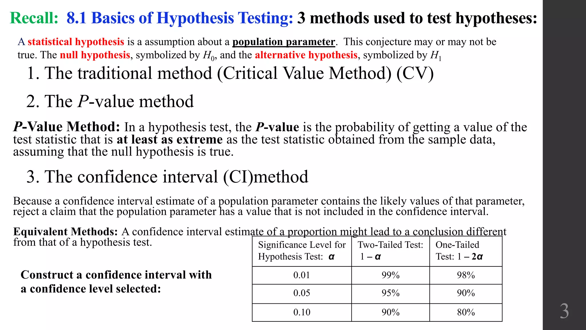
Recall: 8.1 Basics of Hypothesis Testing: 3 methods used to test hypotheses:
3
Construct a confidence interval with
a confidence level selected:
Significance Level for
Hypothesis Test: α
Two-Tailed Test:
1 – α
One-Tailed
Test: 1 – 2α
0.01 99% 98%
0.05 95% 90%
0.10 90% 80%
A statistical hypothesis is a assumption about a population parameter. This conjecture may or may not be
true. The null hypothesis, symbolized by H0, and the alternative hypothesis, symbolized by H1
4
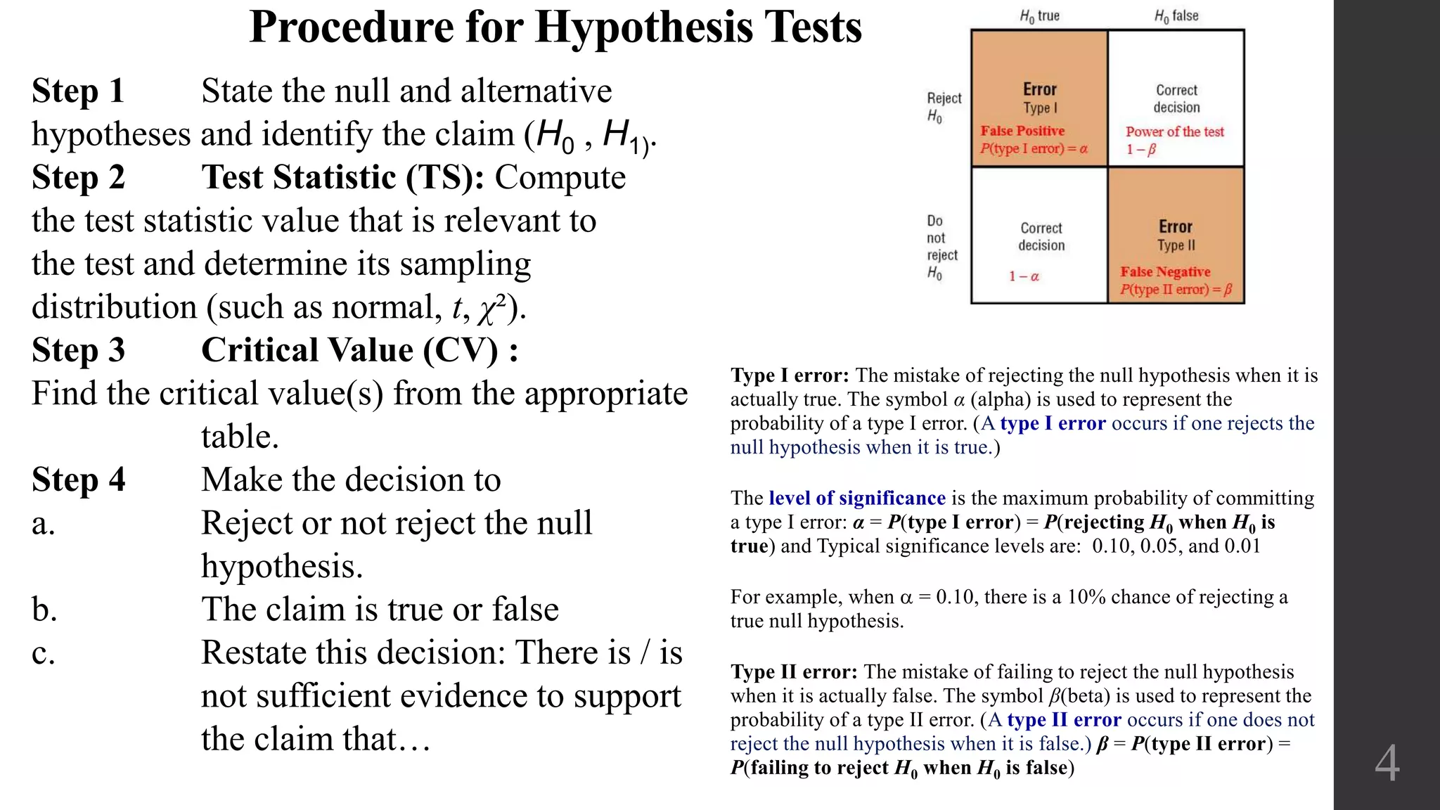
Type I error: The mistake of rejecting the null hypothesis when it is
actually true. The symbol α (alpha) is used to represent the
probability of a type I error. (A type I error occurs if one rejects the
null hypothesis when it is true.)
The level of significance is the maximum probability of committing
a type I error: α = P(type I error) = P(rejecting H0 when H0 is
true) and Typical significance levels are: 0.10, 0.05, and 0.01
For example, when a = 0.10, there is a 10% chance of rejecting a
true null hypothesis.
Type II error: The mistake of failing to reject the null hypothesis
when it is actually false. The symbol β(beta) is used to represent the
probability of a type II error. (A type II error occurs if one does not
reject the null hypothesis when it is false.) β = P(type II error) =
P(failing to reject H0 when H0 is false)
Procedure for Hypothesis Tests
Step 1 State the null and alternative
hypotheses and identify the claim (H0 , H1).
Step 2 Test Statistic (TS): Compute
the test statistic value that is relevant to
the test and determine its sampling
distribution (such as normal, t, χ²).
Step 3 Critical Value (CV) :
Find the critical value(s) from the appropriate
table.
Step 4 Make the decision to
a. Reject or not reject the null
hypothesis.
b. The claim is true or false
c. Restate this decision: There is / is
not sufficient evidence to support
the claim that…
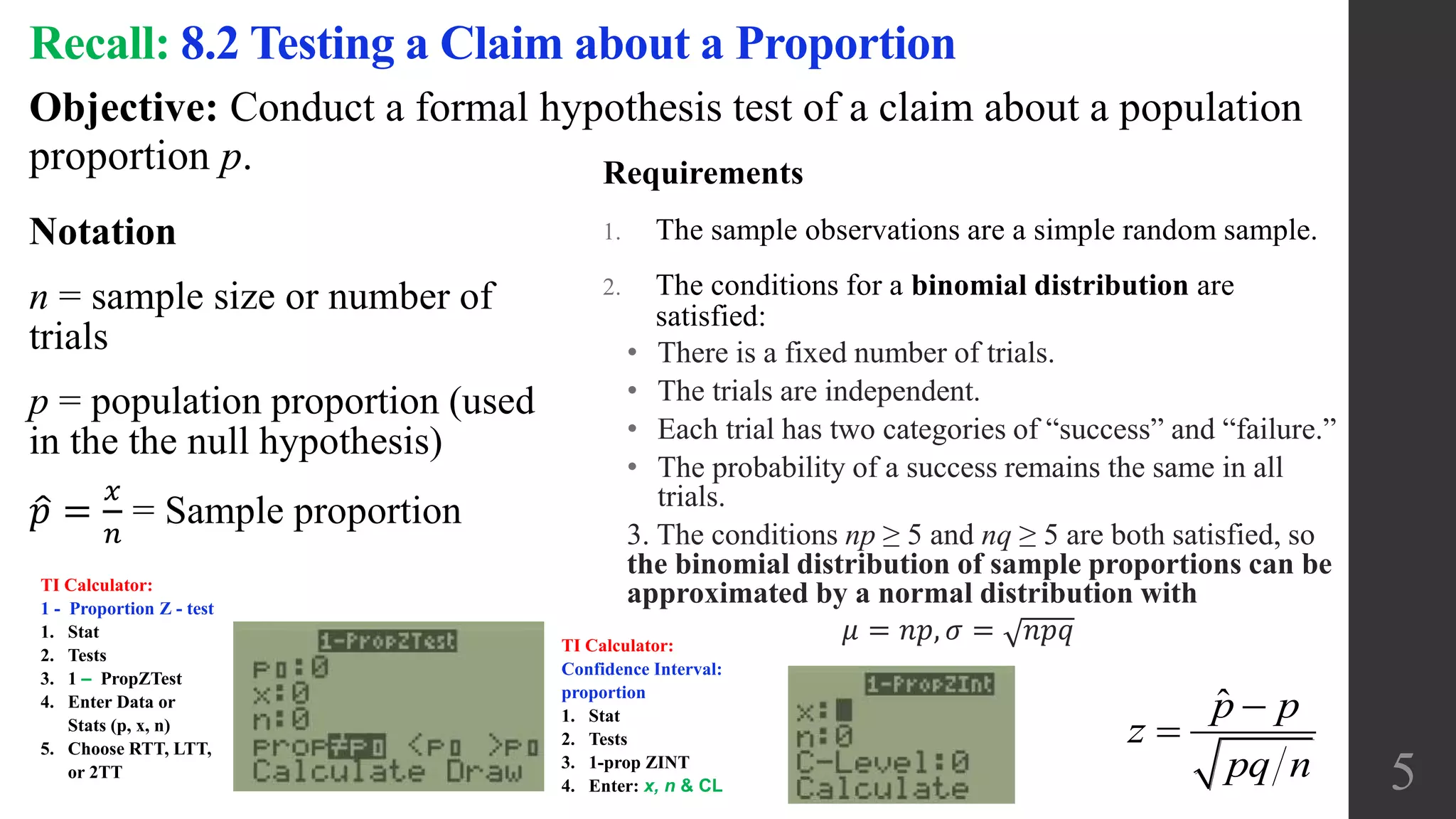
Objective: Conduct a formal hypothesis test of a claim about a population
proportion p.
Recall: 8.2 Testing a Claim about a Proportion
Notation
n = sample size or number of
trials
p = population proportion (used
in the the null hypothesis)
𝑝 =
𝑥
𝑛
= Sample proportion
Requirements
1. The sample observations are a simple random sample.
2. The conditions for a binomial distribution are
satisfied:
• There is a fixed number of trials.
• The trials are independent.
• Each trial has two categories of “success” and “failure.”
• The probability of a success remains the same in all
trials.
3. The conditions np ≥ 5 and nq ≥ 5 are both satisfied, so
the binomial distribution of sample proportions can be
approximated by a normal distribution with
𝜇 = 𝑛𝑝, 𝜎 = 𝑛𝑝𝑞
5
ˆ 

p p
z
pq n
TI Calculator:
1 - Proportion Z - test
1. Stat
2. Tests
3. 1 ‒ PropZTest
4. Enter Data or
Stats (p, x, n)
5. Choose RTT, LTT,
or 2TT
TI Calculator:
Confidence Interval:
proportion
1. Stat
2. Tests
3. 1-prop ZINT
4. Enter: x, n & CL
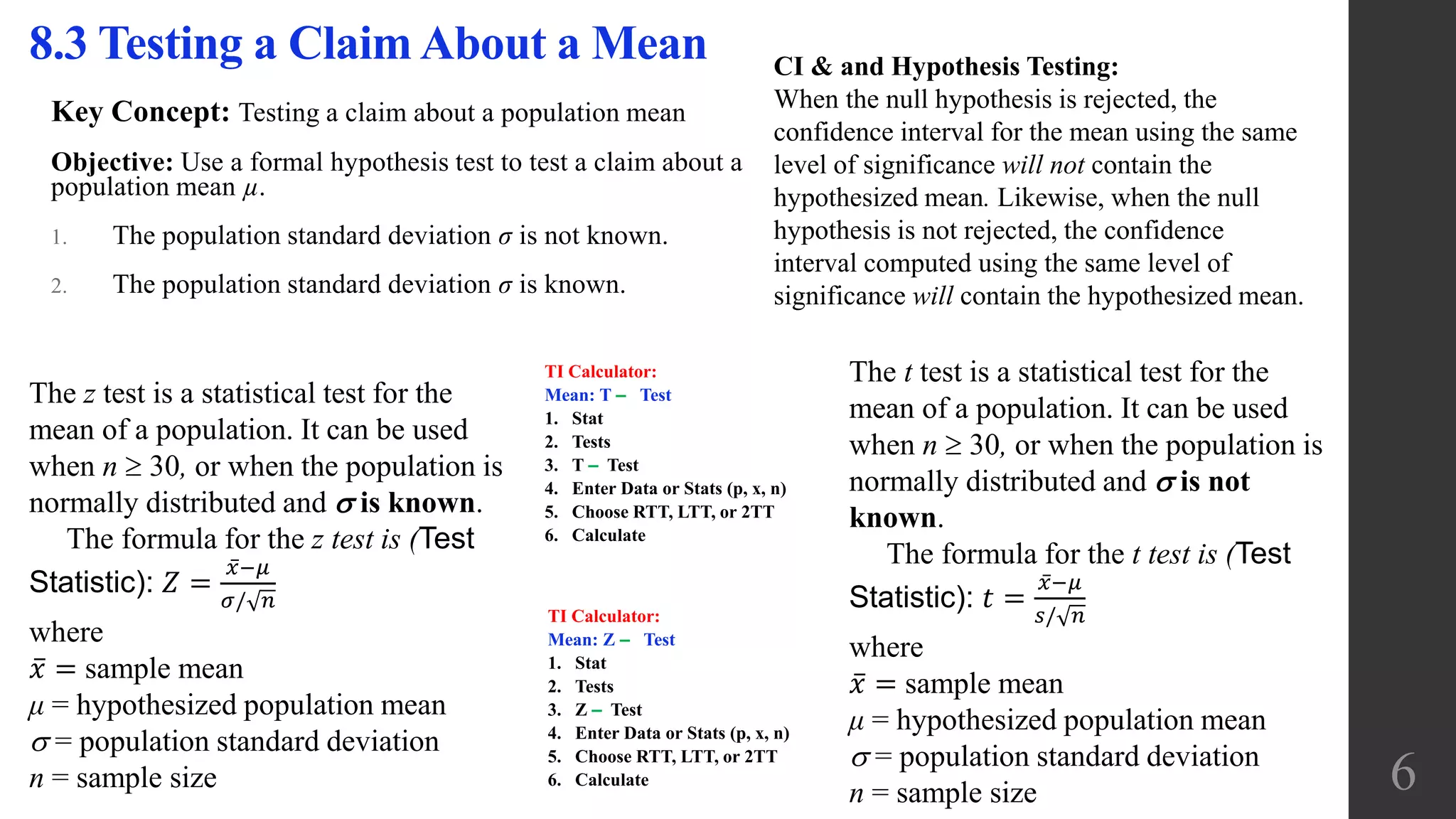
Key Concept: Testing a claim about a population mean
Objective: Use a formal hypothesis test to test a claim about a
population mean µ.
1. The population standard deviation σ is not known.
2. The population standard deviation σ is known.
8.3 Testing a Claim About a Mean
The z test is a statistical test for the
mean of a population. It can be used
when n  30, or when the population is
normally distributed and  is known.
The formula for the z test is (Test
Statistic): 𝑍 =
𝑥−𝜇
𝜎/ 𝑛
where
𝑥 = sample mean
μ = hypothesized population mean
 = population standard deviation
n = sample size
The t test is a statistical test for the
mean of a population. It can be used
when n  30, or when the population is
normally distributed and  is not
known.
The formula for the t test is (Test
Statistic): 𝑡 =
𝑥−𝜇
𝑠/ 𝑛
where
𝑥 = sample mean
μ = hypothesized population mean
 = population standard deviation
n = sample size 6
CI & and Hypothesis Testing:
When the null hypothesis is rejected, the
confidence interval for the mean using the same
level of significance will not contain the
hypothesized mean. Likewise, when the null
hypothesis is not rejected, the confidence
interval computed using the same level of
significance will contain the hypothesized mean.
TI Calculator:
Mean: T ‒ Test
1. Stat
2. Tests
3. T ‒ Test
4. Enter Data or Stats (p, x, n)
5. Choose RTT, LTT, or 2TT
6. Calculate
TI Calculator:
Mean: Z ‒ Test
1. Stat
2. Tests
3. Z ‒ Test
4. Enter Data or Stats (p, x, n)
5. Choose RTT, LTT, or 2TT
6. Calculate
7
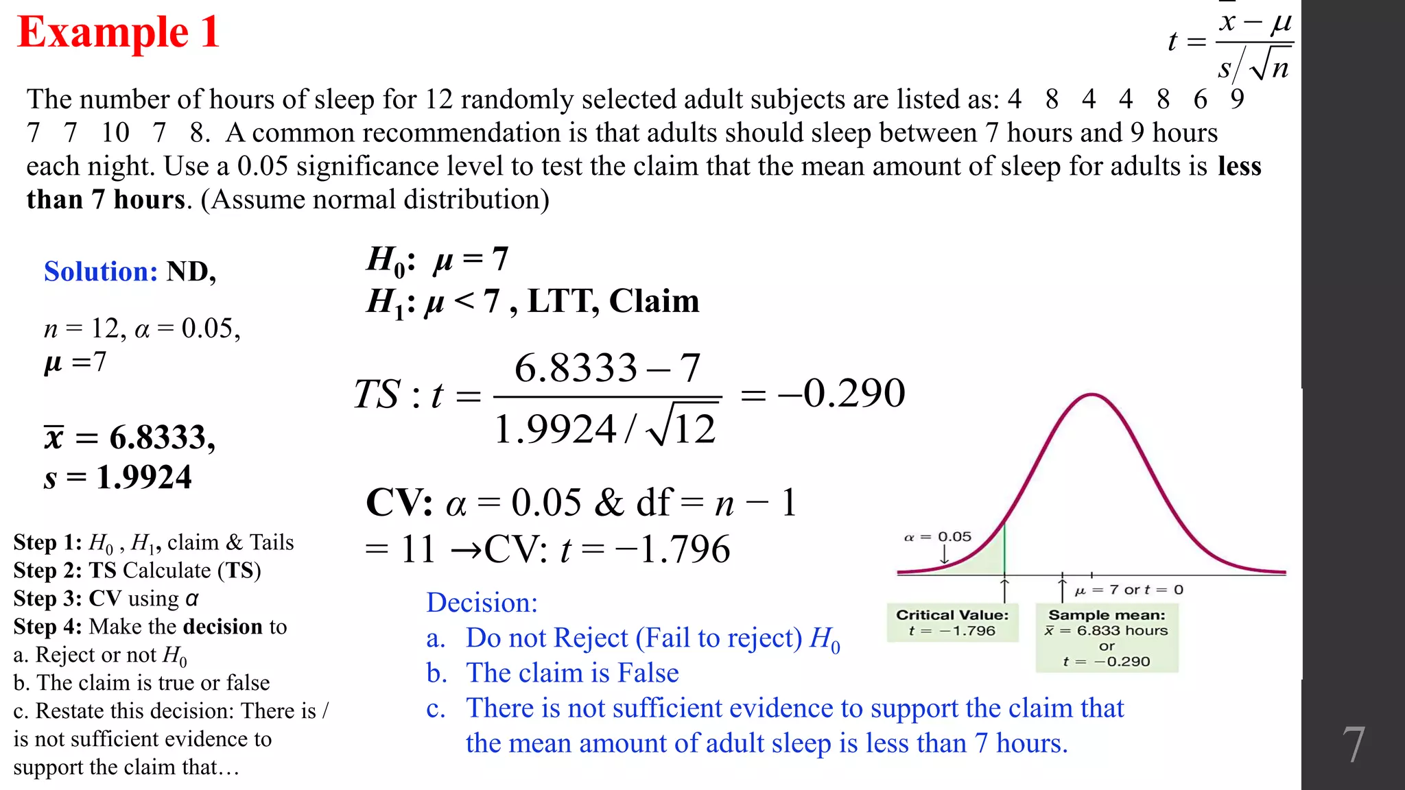
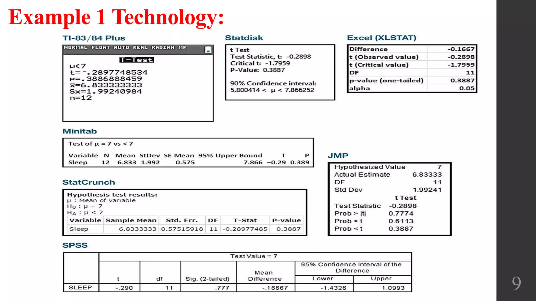
The number of hours of sleep for 12 randomly selected adult subjects are listed as: 4 8 4 4 8 6 9
7 7 10 7 8. A common recommendation is that adults should sleep between 7 hours and 9 hours
each night. Use a 0.05 significance level to test the claim that the mean amount of sleep for adults is less
than 7 hours. (Assume normal distribution)
Example 1
CV: α = 0.05 & df = n − 1
= 11 →CV: t = −1.796
H0: μ = 7
H1: μ < 7 , LTT, Claim
Solution: ND,
n = 12, α = 0.05,
𝝁 =7 6.8333 7
:
1.9924 / 12
TS t

 0.290 
Decision:
a. Do not Reject (Fail to reject) H0
b. The claim is False
c. There is not sufficient evidence to support the claim that
the mean amount of adult sleep is less than 7 hours.
x
t
s n


𝒙 = 6.8333,
s = 1.9924
Step 1: H0 , H1, claim & Tails
Step 2: TS Calculate (TS)
Step 3: CV using α
Step 4: Make the decision to
a. Reject or not H0
b. The claim is true or false
c. Restate this decision: There is /
is not sufficient evidence to
support the claim that…
The P-Values Method
8
Example 1 continued:
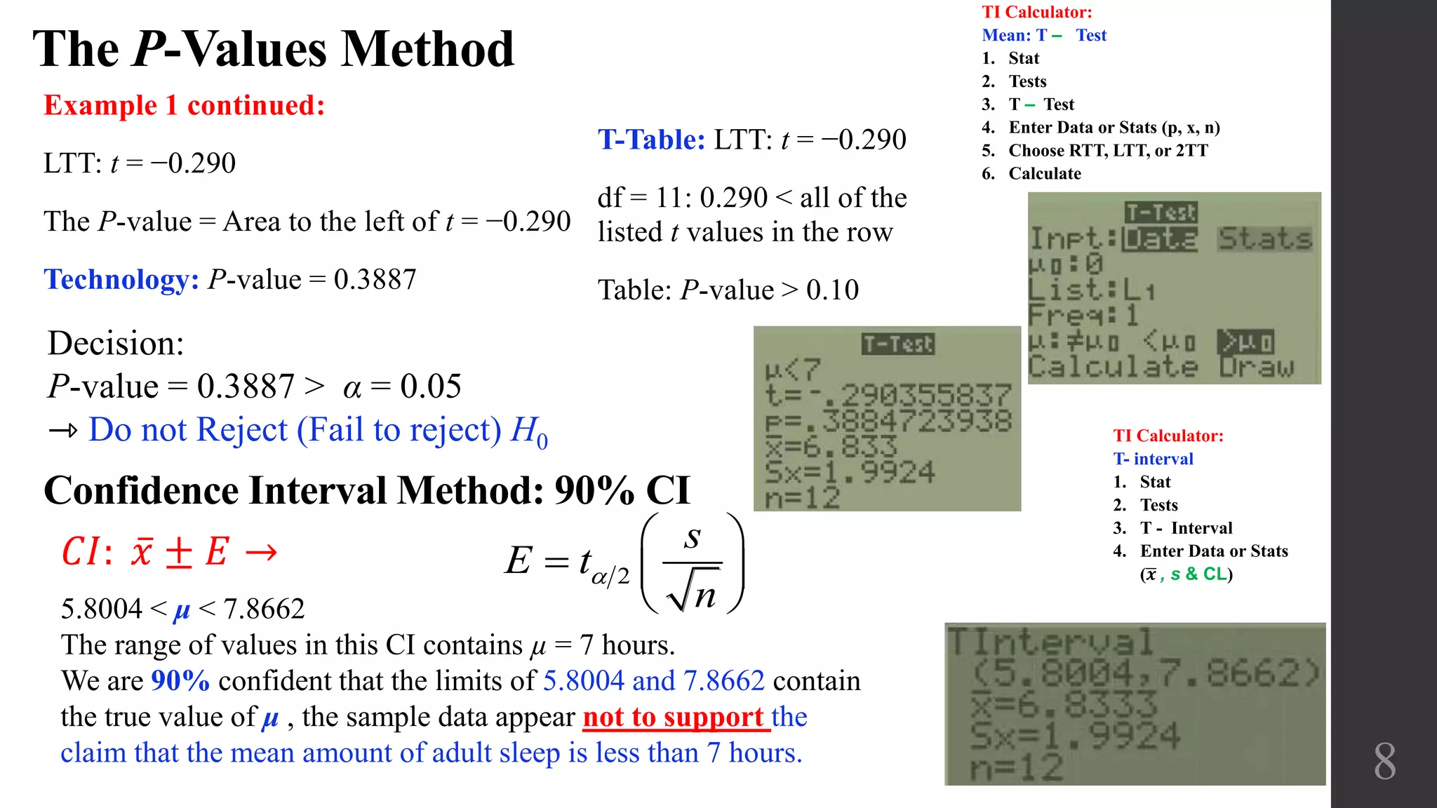
LTT: t = −0.290
The P-value = Area to the left of t = −0.290
Technology: P-value = 0.3887
Decision:
P-value = 0.3887 > α = 0.05
⇾ Do not Reject (Fail to reject) H0
5.8004 < μ < 7.8662
The range of values in this CI contains µ = 7 hours.
We are 90% confident that the limits of 5.8004 and 7.8662 contain
the true value of μ , the sample data appear not to support the
claim that the mean amount of adult sleep is less than 7 hours.
Confidence Interval Method: 90% CI
T-Table: LTT: t = −0.290
df = 11: 0.290 < all of the
listed t values in the row
Table: P-value > 0.10
𝐶𝐼: 𝑥 ± 𝐸 → 2
s
E t
n
a
 
  
 
TI Calculator:
Mean: T ‒ Test
1. Stat
2. Tests
3. T ‒ Test
4. Enter Data or Stats (p, x, n)
5. Choose RTT, LTT, or 2TT
6. Calculate
TI Calculator:
T- interval
1. Stat
2. Tests
3. T - Interval
4. Enter Data or Stats
( 𝒙 , s & CL)
9
Example 1 Technology:
10
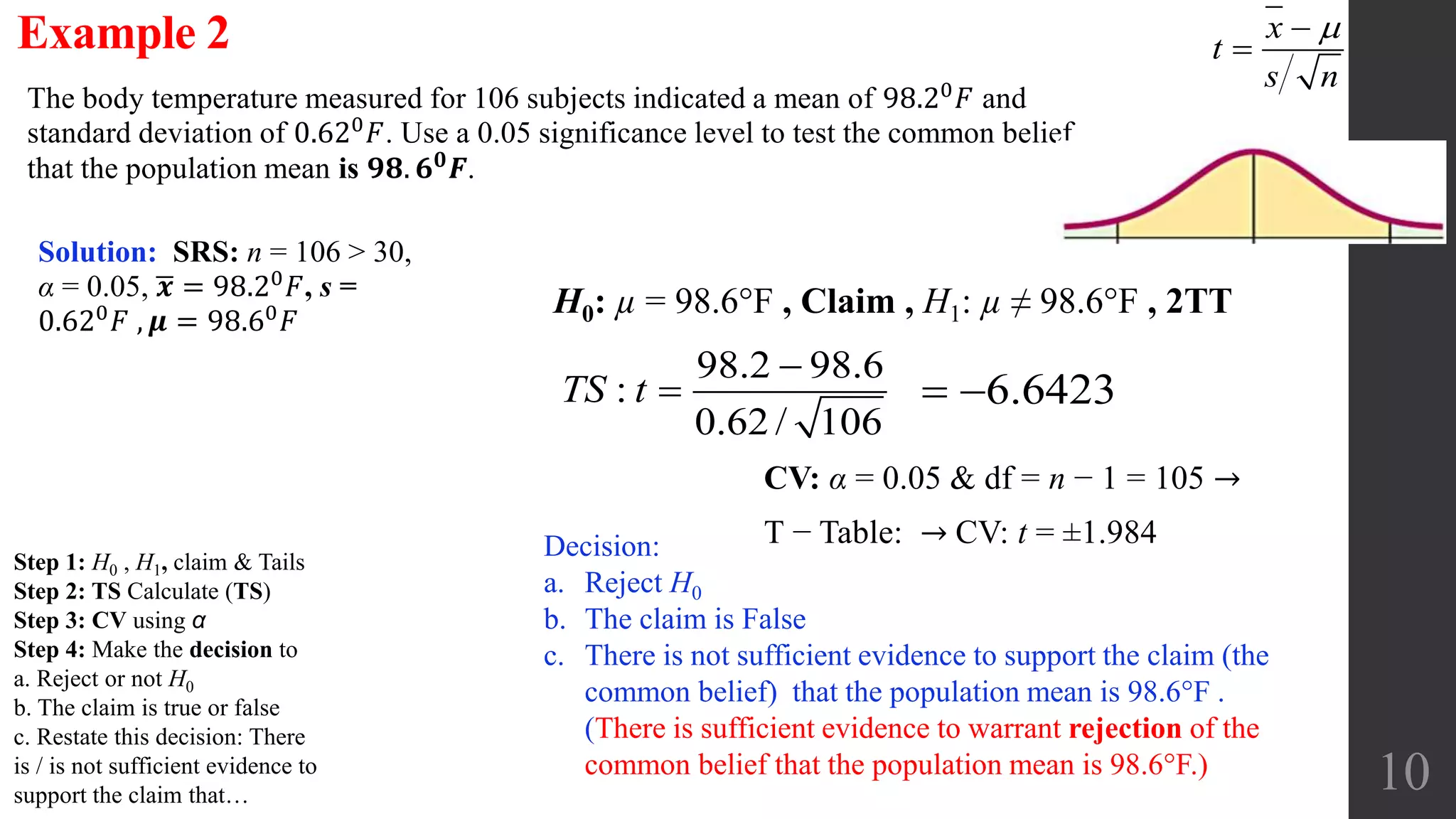
The body temperature measured for 106 subjects indicated a mean of 98.20 𝐹 and
standard deviation of 0.620 𝐹. Use a 0.05 significance level to test the common belief
that the population mean is 𝟗𝟖. 𝟔 𝟎
𝑭.
Example 2
CV: α = 0.05 & df = n − 1 = 105 →
T − Table: → CV: t = ±1.984
H0: µ = 98.6°F , Claim , H1: µ ≠ 98.6°F , 2TT
Solution: SRS: n = 106 > 30,
α = 0.05, 𝒙 = 98.20 𝐹, s =
0.620 𝐹 , 𝝁 = 98.60 𝐹
98.2 98.6
:
0.62 / 106
TS t

 6.6423 
Decision:
a. Reject H0
b. The claim is False
c. There is not sufficient evidence to support the claim (the
common belief) that the population mean is 98.6°F .
(There is sufficient evidence to warrant rejection of the
common belief that the population mean is 98.6°F.)
x
t
s n


Step 1: H0 , H1, claim & Tails
Step 2: TS Calculate (TS)
Step 3: CV using α
Step 4: Make the decision to
a. Reject or not H0
b. The claim is true or false
c. Restate this decision: There
is / is not sufficient evidence to
support the claim that…
The P-Values Method
11
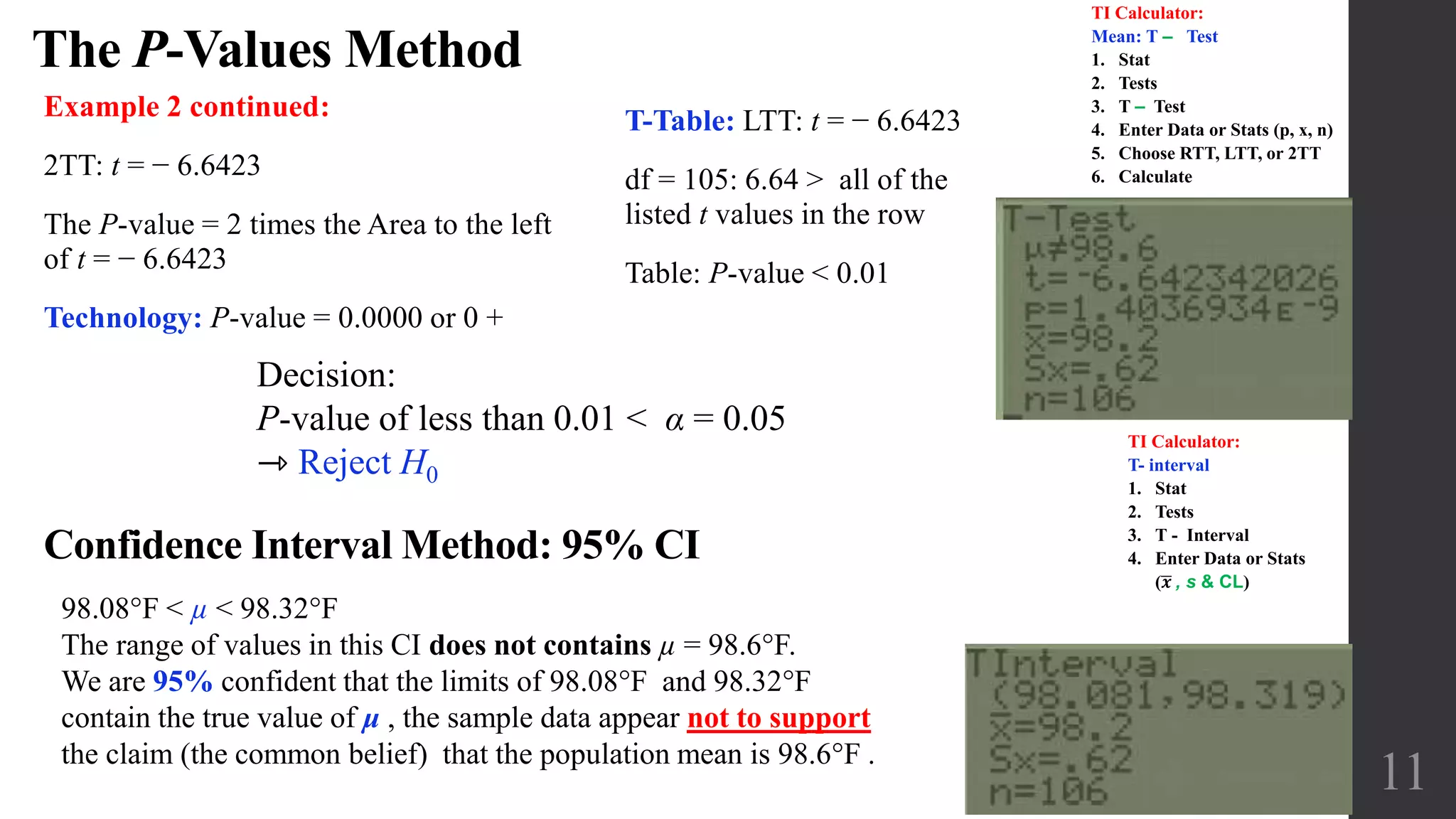
Example 2 continued:
2TT: t = − 6.6423
The P-value = 2 times the Area to the left
of t = − 6.6423
Technology: P-value = 0.0000 or 0 +
Decision:
P-value of less than 0.01 < α = 0.05
⇾ Reject H0
98.08°F < µ < 98.32F
The range of values in this CI does not contains µ = 98.6F.
We are 95% confident that the limits of 98.08°F and 98.32F
contain the true value of μ , the sample data appear not to support
the claim (the common belief) that the population mean is 98.6°F .
Confidence Interval Method: 95% CI
T-Table: LTT: t = − 6.6423
df = 105: 6.64 > all of the
listed t values in the row
Table: P-value < 0.01
TI Calculator:
Mean: T ‒ Test
1. Stat
2. Tests
3. T ‒ Test
4. Enter Data or Stats (p, x, n)
5. Choose RTT, LTT, or 2TT
6. Calculate
TI Calculator:
T- interval
1. Stat
2. Tests
3. T - Interval
4. Enter Data or Stats
( 𝒙 , s & CL)
12
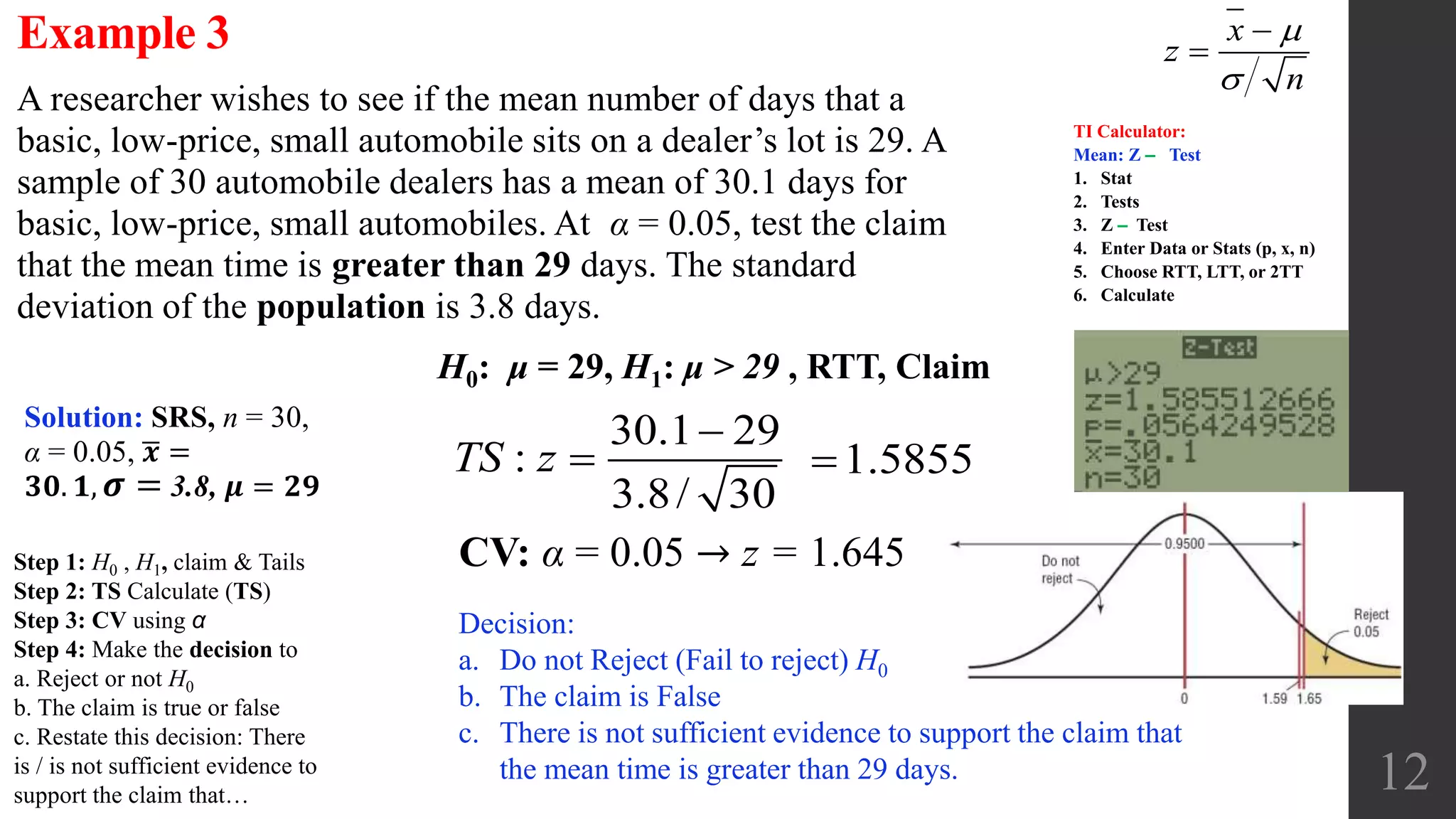
A researcher wishes to see if the mean number of days that a
basic, low-price, small automobile sits on a dealer’s lot is 29. A
sample of 30 automobile dealers has a mean of 30.1 days for
basic, low-price, small automobiles. At α = 0.05, test the claim
that the mean time is greater than 29 days. The standard
deviation of the population is 3.8 days.
Example 3
CV: α = 0.05 → z = 1.645
H0: μ = 29, H1: μ > 29 , RTT, Claim
Solution: SRS, n = 30,
α = 0.05, 𝒙 =
𝟑𝟎. 𝟏, 𝝈 = 3.8, 𝝁 = 𝟐𝟗
30.1 29
:
3.8/ 30
TS z

 1.5855
Decision:
a. Do not Reject (Fail to reject) H0
b. The claim is False
c. There is not sufficient evidence to support the claim that
the mean time is greater than 29 days.
x
z
n




TI Calculator:
Mean: Z ‒ Test
1. Stat
2. Tests
3. Z ‒ Test
4. Enter Data or Stats (p, x, n)
5. Choose RTT, LTT, or 2TT
6. Calculate
Step 1: H0 , H1, claim & Tails
Step 2: TS Calculate (TS)
Step 3: CV using α
Step 4: Make the decision to
a. Reject or not H0
b. The claim is true or false
c. Restate this decision: There
is / is not sufficient evidence to
support the claim that…

Testing a claim about a mean

  • 1.
    Elementary Statistics Chapter 8: HypothesisTesting 8.3 Testing a Claim about a Mean 1
  • 2.
    8.1 Basics ofHypothesis Testing 8.2 Testing a Claim about a Proportion 8.3 Testing a Claim About a Mean 8.4 Testing a Claim About a Standard Deviation or Variance 2 Objectives: • Understand the definitions used in hypothesis testing. • State the null and alternative hypotheses. • State the steps used in hypothesis testing. • Test proportions, using the z test. • Test means when  is known, using the z test. • Test means when  is unknown, using the t test. • Test variances or standard deviations, using the chi-square test. • Test hypotheses, using confidence intervals. Chapter 8: Hypothesis Testing
  • 3.
    1. The traditionalmethod (Critical Value Method) (CV) 2. The P-value method P-Value Method: In a hypothesis test, the P-value is the probability of getting a value of the test statistic that is at least as extreme as the test statistic obtained from the sample data, assuming that the null hypothesis is true. 3. The confidence interval (CI)method Because a confidence interval estimate of a population parameter contains the likely values of that parameter, reject a claim that the population parameter has a value that is not included in the confidence interval. Equivalent Methods: A confidence interval estimate of a proportion might lead to a conclusion different from that of a hypothesis test. Recall: 8.1 Basics of Hypothesis Testing: 3 methods used to test hypotheses: 3 Construct a confidence interval with a confidence level selected: Significance Level for Hypothesis Test: α Two-Tailed Test: 1 – α One-Tailed Test: 1 – 2α 0.01 99% 98% 0.05 95% 90% 0.10 90% 80% A statistical hypothesis is a assumption about a population parameter. This conjecture may or may not be true. The null hypothesis, symbolized by H0, and the alternative hypothesis, symbolized by H1
  • 4.
    4 Type I error:The mistake of rejecting the null hypothesis when it is actually true. The symbol α (alpha) is used to represent the probability of a type I error. (A type I error occurs if one rejects the null hypothesis when it is true.) The level of significance is the maximum probability of committing a type I error: α = P(type I error) = P(rejecting H0 when H0 is true) and Typical significance levels are: 0.10, 0.05, and 0.01 For example, when a = 0.10, there is a 10% chance of rejecting a true null hypothesis. Type II error: The mistake of failing to reject the null hypothesis when it is actually false. The symbol β(beta) is used to represent the probability of a type II error. (A type II error occurs if one does not reject the null hypothesis when it is false.) β = P(type II error) = P(failing to reject H0 when H0 is false) Procedure for Hypothesis Tests Step 1 State the null and alternative hypotheses and identify the claim (H0 , H1). Step 2 Test Statistic (TS): Compute the test statistic value that is relevant to the test and determine its sampling distribution (such as normal, t, χ²). Step 3 Critical Value (CV) : Find the critical value(s) from the appropriate table. Step 4 Make the decision to a. Reject or not reject the null hypothesis. b. The claim is true or false c. Restate this decision: There is / is not sufficient evidence to support the claim that…
  • 5.
    Objective: Conduct aformal hypothesis test of a claim about a population proportion p. Recall: 8.2 Testing a Claim about a Proportion Notation n = sample size or number of trials p = population proportion (used in the the null hypothesis) 𝑝 = 𝑥 𝑛 = Sample proportion Requirements 1. The sample observations are a simple random sample. 2. The conditions for a binomial distribution are satisfied: • There is a fixed number of trials. • The trials are independent. • Each trial has two categories of “success” and “failure.” • The probability of a success remains the same in all trials. 3. The conditions np ≥ 5 and nq ≥ 5 are both satisfied, so the binomial distribution of sample proportions can be approximated by a normal distribution with 𝜇 = 𝑛𝑝, 𝜎 = 𝑛𝑝𝑞 5 ˆ   p p z pq n TI Calculator: 1 - Proportion Z - test 1. Stat 2. Tests 3. 1 ‒ PropZTest 4. Enter Data or Stats (p, x, n) 5. Choose RTT, LTT, or 2TT TI Calculator: Confidence Interval: proportion 1. Stat 2. Tests 3. 1-prop ZINT 4. Enter: x, n & CL
  • 6.
    Key Concept: Testinga claim about a population mean Objective: Use a formal hypothesis test to test a claim about a population mean µ. 1. The population standard deviation σ is not known. 2. The population standard deviation σ is known. 8.3 Testing a Claim About a Mean The z test is a statistical test for the mean of a population. It can be used when n  30, or when the population is normally distributed and  is known. The formula for the z test is (Test Statistic): 𝑍 = 𝑥−𝜇 𝜎/ 𝑛 where 𝑥 = sample mean μ = hypothesized population mean  = population standard deviation n = sample size The t test is a statistical test for the mean of a population. It can be used when n  30, or when the population is normally distributed and  is not known. The formula for the t test is (Test Statistic): 𝑡 = 𝑥−𝜇 𝑠/ 𝑛 where 𝑥 = sample mean μ = hypothesized population mean  = population standard deviation n = sample size 6 CI & and Hypothesis Testing: When the null hypothesis is rejected, the confidence interval for the mean using the same level of significance will not contain the hypothesized mean. Likewise, when the null hypothesis is not rejected, the confidence interval computed using the same level of significance will contain the hypothesized mean. TI Calculator: Mean: T ‒ Test 1. Stat 2. Tests 3. T ‒ Test 4. Enter Data or Stats (p, x, n) 5. Choose RTT, LTT, or 2TT 6. Calculate TI Calculator: Mean: Z ‒ Test 1. Stat 2. Tests 3. Z ‒ Test 4. Enter Data or Stats (p, x, n) 5. Choose RTT, LTT, or 2TT 6. Calculate
  • 7.
    7 The number ofhours of sleep for 12 randomly selected adult subjects are listed as: 4 8 4 4 8 6 9 7 7 10 7 8. A common recommendation is that adults should sleep between 7 hours and 9 hours each night. Use a 0.05 significance level to test the claim that the mean amount of sleep for adults is less than 7 hours. (Assume normal distribution) Example 1 CV: α = 0.05 & df = n − 1 = 11 →CV: t = −1.796 H0: μ = 7 H1: μ < 7 , LTT, Claim Solution: ND, n = 12, α = 0.05, 𝝁 =7 6.8333 7 : 1.9924 / 12 TS t   0.290  Decision: a. Do not Reject (Fail to reject) H0 b. The claim is False c. There is not sufficient evidence to support the claim that the mean amount of adult sleep is less than 7 hours. x t s n   𝒙 = 6.8333, s = 1.9924 Step 1: H0 , H1, claim & Tails Step 2: TS Calculate (TS) Step 3: CV using α Step 4: Make the decision to a. Reject or not H0 b. The claim is true or false c. Restate this decision: There is / is not sufficient evidence to support the claim that…
  • 8.
    The P-Values Method 8 Example1 continued: LTT: t = −0.290 The P-value = Area to the left of t = −0.290 Technology: P-value = 0.3887 Decision: P-value = 0.3887 > α = 0.05 ⇾ Do not Reject (Fail to reject) H0 5.8004 < μ < 7.8662 The range of values in this CI contains µ = 7 hours. We are 90% confident that the limits of 5.8004 and 7.8662 contain the true value of μ , the sample data appear not to support the claim that the mean amount of adult sleep is less than 7 hours. Confidence Interval Method: 90% CI T-Table: LTT: t = −0.290 df = 11: 0.290 < all of the listed t values in the row Table: P-value > 0.10 𝐶𝐼: 𝑥 ± 𝐸 → 2 s E t n a        TI Calculator: Mean: T ‒ Test 1. Stat 2. Tests 3. T ‒ Test 4. Enter Data or Stats (p, x, n) 5. Choose RTT, LTT, or 2TT 6. Calculate TI Calculator: T- interval 1. Stat 2. Tests 3. T - Interval 4. Enter Data or Stats ( 𝒙 , s & CL)
  • 9.
  • 10.
    10 The body temperaturemeasured for 106 subjects indicated a mean of 98.20 𝐹 and standard deviation of 0.620 𝐹. Use a 0.05 significance level to test the common belief that the population mean is 𝟗𝟖. 𝟔 𝟎 𝑭. Example 2 CV: α = 0.05 & df = n − 1 = 105 → T − Table: → CV: t = ±1.984 H0: µ = 98.6°F , Claim , H1: µ ≠ 98.6°F , 2TT Solution: SRS: n = 106 > 30, α = 0.05, 𝒙 = 98.20 𝐹, s = 0.620 𝐹 , 𝝁 = 98.60 𝐹 98.2 98.6 : 0.62 / 106 TS t   6.6423  Decision: a. Reject H0 b. The claim is False c. There is not sufficient evidence to support the claim (the common belief) that the population mean is 98.6°F . (There is sufficient evidence to warrant rejection of the common belief that the population mean is 98.6°F.) x t s n   Step 1: H0 , H1, claim & Tails Step 2: TS Calculate (TS) Step 3: CV using α Step 4: Make the decision to a. Reject or not H0 b. The claim is true or false c. Restate this decision: There is / is not sufficient evidence to support the claim that…
  • 11.
    The P-Values Method 11 Example2 continued: 2TT: t = − 6.6423 The P-value = 2 times the Area to the left of t = − 6.6423 Technology: P-value = 0.0000 or 0 + Decision: P-value of less than 0.01 < α = 0.05 ⇾ Reject H0 98.08°F < µ < 98.32F The range of values in this CI does not contains µ = 98.6F. We are 95% confident that the limits of 98.08°F and 98.32F contain the true value of μ , the sample data appear not to support the claim (the common belief) that the population mean is 98.6°F . Confidence Interval Method: 95% CI T-Table: LTT: t = − 6.6423 df = 105: 6.64 > all of the listed t values in the row Table: P-value < 0.01 TI Calculator: Mean: T ‒ Test 1. Stat 2. Tests 3. T ‒ Test 4. Enter Data or Stats (p, x, n) 5. Choose RTT, LTT, or 2TT 6. Calculate TI Calculator: T- interval 1. Stat 2. Tests 3. T - Interval 4. Enter Data or Stats ( 𝒙 , s & CL)
  • 12.
    12 A researcher wishesto see if the mean number of days that a basic, low-price, small automobile sits on a dealer’s lot is 29. A sample of 30 automobile dealers has a mean of 30.1 days for basic, low-price, small automobiles. At α = 0.05, test the claim that the mean time is greater than 29 days. The standard deviation of the population is 3.8 days. Example 3 CV: α = 0.05 → z = 1.645 H0: μ = 29, H1: μ > 29 , RTT, Claim Solution: SRS, n = 30, α = 0.05, 𝒙 = 𝟑𝟎. 𝟏, 𝝈 = 3.8, 𝝁 = 𝟐𝟗 30.1 29 : 3.8/ 30 TS z   1.5855 Decision: a. Do not Reject (Fail to reject) H0 b. The claim is False c. There is not sufficient evidence to support the claim that the mean time is greater than 29 days. x z n     TI Calculator: Mean: Z ‒ Test 1. Stat 2. Tests 3. Z ‒ Test 4. Enter Data or Stats (p, x, n) 5. Choose RTT, LTT, or 2TT 6. Calculate Step 1: H0 , H1, claim & Tails Step 2: TS Calculate (TS) Step 3: CV using α Step 4: Make the decision to a. Reject or not H0 b. The claim is true or false c. Restate this decision: There is / is not sufficient evidence to support the claim that…