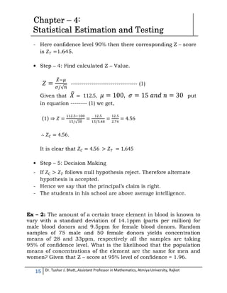
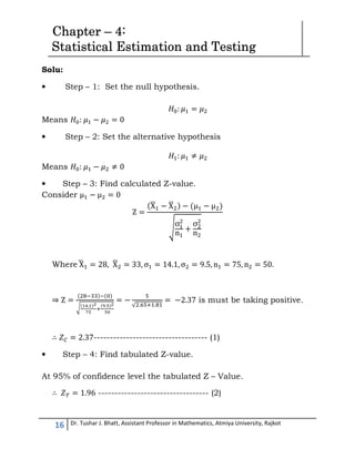
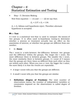
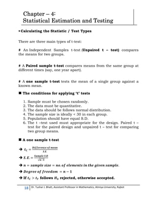
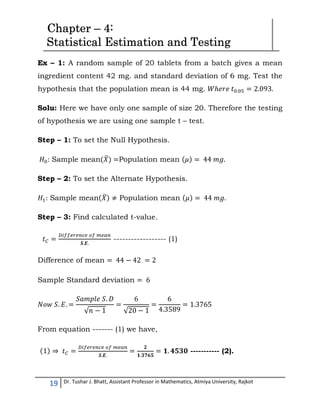
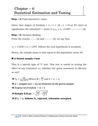
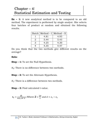
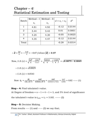
The Statistical Inference is the process of drawing conclusions about on underlying population based on a sample or subset of the data.
In most cases, it is not practical to obtain all the measurements in a given population.
The statistical inference is deals with decision problems. There are two types of decision problems as mentioned below:
(i) Problems of estimation and
(ii) Test of hypotheses
In the problem of estimation, we must determine the value of parameter(s), while in test of hypothesis we must decide whether to accept or reject a specific value(s) of a parameter(s).
Regression analysis is a statistical technique used to estimate the relationships between variables. It allows one to predict the value of a dependent variable based on the value of one or more independent variables. The document discusses simple linear regression, where there is one independent variable, as well as multiple linear regression which involves two or more independent variables. Examples of linear relationships that can be modeled using regression analysis include price vs. quantity, sales vs. advertising, and crop yield vs. fertilizer usage. The key methods for performing regression analysis covered in the document are least squares regression and regressions based on deviations from the mean.
The document discusses the paired samples t-test, which is used to compare two sets of measurements made on the same individuals. It notes that this test is appropriate when there are two correlated distributions, such as pre-test and post-test scores from the same people. The null hypothesis is that there is no difference between the pairs. The test calculates the differences between pairs, sums them, and divides this by the standard error of the differences to obtain a t-value, which can be compared to critical values to determine if the null hypothesis can be rejected.
The document provides an introduction to regression analysis and performing regression using SPSS. It discusses key concepts like dependent and independent variables, assumptions of regression like linearity and homoscedasticity. It explains how to calculate regression coefficients using the method of least squares and how to perform regression analysis in SPSS, including selecting variables and interpreting the output.
This document discusses measures of central tendency and variability in descriptive statistics. It defines and provides formulas for calculating the mean, median, and mode as measures of central tendency. The mean is the most useful measure and is calculated by summing all values and dividing by the total number of observations. Variability refers to how spread out or clustered the data values are and is measured by calculations like the range, variance, and standard deviation. The standard deviation is specifically defined as the average deviation of the data from the mean and is considered the best single measure of variability.
The PPT covered the distinguish between discrete and continuous distribution. Detailed explanation of the types of discrete distributions such as binomial distribution, Poisson distribution & Hyper-geometric distribution.
Hypothesis is usually considered as the principal instrument in research and quality control. Its main function is to suggest new experiments and observations. In fact, many experiments are carried out with the deliberate object of testing hypothesis. Decision makers often face situations wherein they are interested in testing hypothesis on the basis of available information and then take decisions on the basis of such testing. In Six –Sigma methodology, hypothesis testing is a tool of substance and used in analysis phase of the six sigma project so that improvement can be done in right direction
This document discusses types of probability and provides definitions and examples of key probability concepts. It begins with an introduction to probability theory and its applications. The document then defines terms like random experiments, sample spaces, events, favorable events, mutually exclusive events, and independent events. It describes three approaches to measuring probability: classical, frequency, and axiomatic. It concludes with theorems of probability and references.
This document outlines basic probability concepts, including definitions of probability, views of probability (objective and subjective), and elementary properties. It discusses calculating probabilities of events from data in tables, including unconditional/marginal probabilities, conditional probabilities, and joint probabilities. Rules of probability are presented, including the multiplicative rule that the joint probability of two events is equal to the product of the marginal probability of one event and the conditional probability of the other event given the first event. Examples are provided to illustrate key concepts.
This document outlines the process of hypothesis testing. It begins with defining key terms like the null hypothesis (H0), alternative hypothesis (H1), significance level, test statistic, critical value, and decision rule. It then explains the steps involved: 1) setting up H0 and H1, 2) choosing a significance level, 3) calculating the test statistic, 4) finding the critical value, and 5) making a decision by comparing the test statistic and critical value. The overall goal of hypothesis testing is to evaluate claims about a population parameter based on a sample's data.
If everything were the same, we would have no need of statistics. But, people's heights, ages, etc., do vary. We often need to measure the extent to which scores in a dataset differ from each other. Such a measure is called the dispersion of a distribution.
Degree of freedom refers to the number of independent pieces of information used to calculate a statistic. In an example where heights of 5 students were measured, taking a single sample of 1 student's height of 8 feet to calculate variance would have 1 degree of freedom. Taking 2 independent samples of heights 8 feet and 5 feet would have 2 degrees of freedom. When estimating the population mean from samples to then calculate variance, the degrees of freedom is the number of samples minus 1, as the values are not fully independent after estimating the mean.
Hypothesis testing , T test , chi square test, z test Irfan Ullah
- The document discusses hypothesis testing and the p-value approach, which involves specifying the null and alternative hypotheses, calculating a test statistic, determining the p-value, and comparing it to the significance level α to determine whether to reject or accept the null hypothesis.
- It also discusses type I and type II errors, degrees of freedom as the number of independent pieces of information, and chi-square and t-tests as statistical tests.
This document provides an overview of statistical estimation and inference. It discusses point estimation, which provides a single value to estimate an unknown population parameter, and interval estimation, which gives a range of plausible values for the parameter. The key aspects of interval estimation are confidence intervals, which provide a probability statement about where the true population parameter lies. The document also covers important concepts like sampling distributions, the central limit theorem, and factors that influence the width of a confidence interval like sample size. Examples are provided to demonstrate calculating point estimates, confidence intervals, and dealing with independent samples.
Descriptive statistics is used to describe and summarize key characteristics of a data set. Commonly used measures include central tendency, such as the mean, median, and mode, and measures of dispersion like range, interquartile range, standard deviation, and variance. The mean is the average value calculated by summing all values and dividing by the number of values. The median is the middle value when data is arranged in order. The mode is the most frequently occurring value. Measures of dispersion describe how spread out the data is, such as the difference between highest and lowest values (range) or how close values are to the average (standard deviation).
- Hypothesis testing involves evaluating claims about population parameters by comparing a null hypothesis to an alternative hypothesis.
- The null hypothesis states that there is no difference or effect, while the alternative hypothesis states that a difference or effect exists.
- There are three main methods for hypothesis testing: the critical value method which separates a critical region from a noncritical region, the p-value method which calculates the probability of obtaining a test statistic at least as extreme as the sample test statistic assuming the null is true, and the confidence interval method which rejects claims not included in the confidence interval.
- The steps of hypothesis testing are to state the hypotheses, calculate the test statistic, find the critical value, make a decision to reject
The document provides information about the binomial distribution, including its definition, assumptions, and properties. The binomial distribution expresses the probability of success/failure outcomes from Bernoulli trials. It assumes a fixed number of independent trials, a constant probability of success on each trial, and only two possible outcomes per trial (success or failure). The mean and variance of the binomial distribution are provided. Examples are given to demonstrate how to calculate binomial probabilities.
Measure of dispersion has two types Absolute measure and Graphical measure. There are other different types in there.
In this slide the discussed points are:
1. Dispersion & it's types
2. Definition
3. Use
4. Merits
5. Demerits
6. Formula & math
7. Graph and pictures
8. Real life application.
The document discusses simple linear regression. It defines key terms like regression equation, regression line, slope, intercept, residuals, and residual plot. It provides examples of using sample data to generate a regression equation and evaluating that regression model. Specifically, it shows generating a regression equation from bivariate data, checking assumptions visually through scatter plots and residual plots, and interpreting the slope as the marginal change in the response variable from a one unit change in the explanatory variable.
The document discusses regression analysis, including definitions, uses, calculating regression equations from data, graphing regression lines, the standard error of estimate, and limitations. Regression analysis is a statistical technique used to understand the relationship between variables and allow for predictions. The document provides examples of calculating regression equations from various data sets and determining the standard error of estimate.
The document presents the results of a simple linear regression analysis conducted by a black belt to predict the number of calls answered (dependent variable) based on staffing levels (independent variable) using data collected over 240 samples in a call center. The regression equation found 83.4% of the variation in calls answered was explained by staffing levels. Notable outliers and leverage points were identified that could impact the strength of the predicted relationship between calls answered and staffing.
This document discusses regression analysis techniques. It defines regression as the tendency for estimated values to be close to actual values. Regression analysis investigates the relationship between variables, with the independent variable influencing the dependent variable. There are three main types of regression: linear regression which uses a linear equation to model the relationship between one independent and one dependent variable; logistic regression which predicts the probability of a binary outcome using multiple independent variables; and nonlinear regression which models any non-linear relationship between variables. The document provides examples of using linear and logistic regression and discusses their key assumptions and calculations.
This document provides an overview of regression analysis, including:
- Regression analysis measures the average relationship between variables to predict dependent variables from independent variables and show relationships.
- It is widely used in business to predict things like production, prices, and profits. It is also used in sociological and economic studies.
- There are three main methods for studying regression: least squares method, deviations from means method, and deviations from assumed means method. Examples are provided of calculating regression equations for bivariate data using each method.
This document discusses key concepts in statistical estimation including:
- Estimation involves using sample data to infer properties of the population by calculating point estimates and interval estimates.
- A point estimate is a single value that estimates an unknown population parameter, while an interval estimate provides a range of plausible values for the parameter.
- A confidence interval gives the probability that the interval calculated from the sample data contains the true population parameter. Common confidence intervals are 95% confidence intervals.
- Formulas for confidence intervals depend on whether the population standard deviation is known or unknown, and the sample size.
This document discusses various laws of probability including addition law, multiplication law, and binomial law. It provides examples of how to calculate probabilities using these laws, such as calculating the probability of mutually exclusive events using addition law. It also discusses key probability concepts like marginal probability, joint probability, conditional probability, sensitivity, specificity, predictive values, and likelihood ratios.
Regression analysis is a statistical technique for investigating relationships between variables. Simple linear regression defines a relationship between two variables (X and Y) using a best-fit straight line. Multiple regression extends this to model relationships between a dependent variable Y and multiple independent variables (X1, X2, etc.). Regression coefficients are estimated to define the regression equation, and R-squared and the standard error can be used to assess the goodness of fit of the regression model to the data. Regression analysis has applications in pharmaceutical experimentation such as analyzing standard curves for drug analysis.
The document discusses regression analysis and its key concepts. Regression analysis is used to understand the relationship between two or more variables and make predictions. There are two main types: simple linear regression, which involves two variables, and multiple regression, which involves more than two variables. Regression lines show the average relationship between the variables and can be used to predict outcomes. The regression coefficients measure the change in the dependent variable for a unit change in the independent variable. The standard error of the estimate indicates how close the data points are to the regression line.
What is statistical analysis? It's the science of collecting, exploring and presenting large amounts of data to discover underlying patterns and trends. Statistics are applied every day – in research, industry and government – to become more scientific about decisions that need to be made.
Please Subscribe to this Channel for more solutions and lectures
http://www.youtube.com/onlineteaching
Chapter 8: Hypothesis Testing
8.3: Testing a Claim About a Mean
Inferential statistics are used to draw conclusions about populations based on samples. The two primary inferential methods are estimation and hypothesis testing. Estimation involves using sample statistics to estimate unknown population parameters, such as means or proportions. Interval estimation provides a range of plausible values for the population parameter based on the sample data and a level of confidence, such as a 95% confidence interval. The width of the confidence interval depends on factors like the sample size, standard deviation, and desired confidence level.
Please Subscribe to this Channel for more solutions and lectures
http://www.youtube.com/onlineteaching
Chapter 7: Estimating Parameters and Determining Sample Sizes
7.2: Estimating a Population Mean
The document discusses sample size determination for clinical and epidemiological research. It explains that proper sample size is important for validity, accuracy, and reliability of research findings. Key factors to consider in sample size calculations include the study objective, details of the intervention, outcomes, covariates, research design, and study subjects. Precision analysis and power analysis are two common approaches, with power analysis being most suitable for studies aiming to detect an effect. The document provides formulas and examples for calculating sample sizes for comparative and descriptive studies with both continuous and dichotomous outcomes. It also discusses the concepts of type I and II errors and their relationship to statistical power.
This document provides an overview of key concepts related to statistical estimation and hypothesis testing, including:
- The difference between point estimation and interval estimation, and examples like confidence intervals for the mean and proportion.
- How to calculate and interpret confidence intervals.
- The roles of the null and alternative hypotheses in hypothesis testing and how to interpret p-values.
- Types I and II errors and how the significance level affects these.
- When to use parametric vs. nonparametric tests and examples of selected nonparametric tests like the chi-square test of goodness of fit.
This document discusses confidence intervals, which are interval estimates of population parameters that indicate the reliability of sample estimates. The document defines confidence intervals and explains how they are constructed. It also discusses point estimates versus interval estimates and describes how to calculate confidence intervals for means, proportions, and when the population standard deviation is unknown using the t-distribution. Examples are provided to illustrate how to construct confidence intervals in different situations.
Running head COURSE PROJECT –PHASE 3 COURSE PROJECT –PHASE 3.docxsusanschei
Running head: COURSE PROJECT –PHASE 3
COURSE PROJECT –PHASE 3
Course Project –Phase 3
Name: Rodney Wheeler
Institution: Rasmussen College
Course: STA3215 Section 01 Inferential Statistics and Analytics
Date: 03/04/17
Course Project –Phase 3
The primary goal of statistics is to conduct a hypothesis. A hypothesis is a prediction about something; hypothesis testing is done to ascertain if a sampled proportion differs from a specified population. For the test to be valid eight steps are conducted to ensure the results are up to par (Lora M. and Richard J. Cook., 2009);
Step One -Identify and come up with a research question, this helps the researcher narrow down to what they want to test.For instance, is the number of patients admitted with infectious disease less than 65 years of age? Such questions are important as they help one in looking for the necessary data and conduct the test efficiently
Step Two-Ascertain that some expectations are met: The method of research used is Simple random sampling, the resultant outcome is only one, and the population is triple the sample size in question
Step Three-State the two types of hypothesis: Identify the null and alternative hypothesis. Null hypothesis shows equality while alternative does not.
Step Four-Determine a definite significant level that is the odds of refuting a null hypothesis through use of alpha
Step Five-Calculate the test statistic, this are constant values that are calculated from the available data when conducting a hypothesis test
Step Six-Change the test statistic into a P value; A p-value is the possibility that a selected sample would differ with the obtained one. It differs depending on the test used and is determined by use of the normal distribution table
Step Seven-Choose between the null and alternative hypothesis, this is where one has to determine whether the stated research question is correct. If the p-value is greater than the standardized value, the null hypothesis should be rejected
Step Eight-Creating a conclusion of your Research Question, determine whether or not the set values are sufficient evidence in confirming your research.
The p-value is the better approach as computation of one value is required to conduct the test, the critical approach is cumbersome as one has to compute the test statistic and also find the key value of the significance level
Question two
1. Ho:p>=65;Ha p<65
2. The test is left tailed since the sample proportion is less than the hypothesized population proportion
3. The test statistics to be used is the t test since the standard deviation is unknown.
4. =-2.79
5. Degree of freedom is 60-1=59as observed from the t table the p- value is 0.05
6. 0.5-0.05=0.45 critical value is -1.6
Subtracting alpha from the standard value of 0.5 then looking for the resultant difference in the z table.
7. Reject the null hypothesis since the test statistic is less than -1.6 which is the critical value.
8. There is sufficient evidenc ...
1) The document discusses hypothesis testing of claims about population means and proportions. It provides examples of testing claims about means using z-tests when the population standard deviation is known and t-tests when it is unknown.
2) Example 1 uses a t-test to test the claim that the mean amount of sleep for adults is less than 7 hours, finding no significant evidence to reject the null hypothesis.
3) Example 2 uses a z-test to reject the common belief that the population mean body temperature is 98.6°F, finding significant evidence against the null hypothesis.
4) Example 3 uses a z-test to find no significant evidence that the mean number of days a car sits on a dealer
This document introduces parametric tests and provides information about the t-test. It defines parametric tests as those applied to normally distributed data measured on interval or ratio scales. Parametric tests make inferences about the parameters of the probability distribution from which the sample data were drawn. Examples of common parametric tests are provided, including the t-test. The t-test is used to compare two means from independent samples or correlated samples. Steps for conducting a t-test are outlined, including calculating the t-statistic and making decisions based on critical t-values. Two examples of using a t-test on experimental data are shown.
This document defines biometry and summarizes statistical methods for estimating population parameters from sample data. It begins by defining biometry as the application of statistical methods to biological problems, involving the measurement of life. It then discusses two types of estimation: point estimation, which provides a single value as an estimate, and interval estimation, which provides a range of values that the parameter is expected to fall within at a given confidence level. The document provides formulas and examples for constructing confidence intervals to estimate a single mean, the difference between two population means, and other parameters, depending on whether the population standard deviation is known or estimated from sample data, and whether sample sizes are large or small.
This document defines biometry and provides examples of its applications. It begins by defining statistics and its uses in collecting and analyzing numerical data. It then discusses the following key points:
- Biometry refers to the application of statistical methods to solve biological problems, through measuring and analyzing life-related data.
- Early statistical methods for experimental design originated in agricultural research, pioneered by Ronald Fisher in his work analyzing wheat experiments. He developed random assignment, balancing treatments, determining optimal replication, and accounting for variability.
- Biometry is used to estimate population parameters like means from sample data using techniques like point estimation, interval estimation, and hypothesis testing. Estimation accounts for variables like sample size, known or estimated standard
Testing of Hypothesis and Goodness of Fit
This document discusses hypothesis testing and goodness of fit. It defines hypothesis testing as a procedure to determine if sample data agrees with a hypothesized population characteristic. The key steps are stating the null and alternative hypotheses, selecting a significance level, determining the test distribution, defining rejection regions, performing the statistical test, and drawing a conclusion. Common hypothesis tests discussed include the Student's t-test and chi-square test of goodness of fit.
Hypothesis testing involves setting up a null hypothesis and alternative hypothesis, determining a significance level, calculating a test statistic, identifying the critical region, computing the test statistic value based on a sample, and making a decision to reject or fail to reject the null hypothesis. The z-test is used when the sample size is large and the population standard deviation is known, while the t-test is used for small samples when the population standard deviation is unknown. Both tests involve calculating a test statistic and comparing it to critical values to determine if there is sufficient evidence to reject the null hypothesis. Limitations include that the tests only indicate differences and not the reasons for them, and inferences are based on probabilities rather than certainty.
The document discusses experimental and quasi-experimental research methods. It defines key characteristics of experimental research such as random assignment, control and intervention groups, and pre- and post-testing. Issues of internal and external validity are examined. Common statistical analyses for experimental designs are introduced, including t-tests, ANOVA, and multiple regression. Examples of experimental designs like single-group, non-equivalent groups, interrupted time series, and factorial designs are also summarized.
Application of Central Limit Theorem to Study the Student Skills in Verbal, A...theijes
Through this paper we analyses the application of the central limit theorem to study the Verbal, Apptitude and Reasoning skills of students. The planning of teaching is based on the mathematical knowledge about the theorem. The different meanings of this theorem were analyzed using the history of its development and previous research studies related to this theorem. Results at the end of this work will serve to improve the correct application of different elements of meaning for central limit theorem when solving the selected problem and to prepare new proposals to teach statistics to students. The central limit theorem forms the basis of inferential statistics and it would be difficult to overestimate its importance. In a statistical study, the sample mean is used to estimate the population mean. However, the number of different samples (of a given size) that could be taken is extremely large and these different samples would have different means. Some would be lower than the mean of the population and some would be higher.The central limit theorem states that, for samples of size n from a normal population, the distribution of sample means is normal with a mean equal to the mean of the population and a standard deviation equal to the standard deviation of the population divided by the square root of the sample size. (For suitably large sample sizes, the central limit theorem also applies to populations whose distributions are not normal.)
This document provides an overview of sampling theory and statistical analysis. It discusses different sampling methods, important sampling terms, and statistical tests. The key points are:
1) There are two ways to collect statistical data - a complete enumeration (census) or a sample survey. A sample is a portion of a population that is examined to estimate population characteristics.
2) Common sampling methods include simple random sampling, systematic sampling, stratified sampling, cluster sampling, quota sampling, and purposive sampling.
3) Important terms include parameters, statistics, sampling distributions, and statistical inferences about populations based on sample data.
4) Statistical tests covered include hypothesis testing, types of errors, test statistics, critical values,
Estimation and hypothesis testing 1 (graduate statistics2)Harve Abella
This document discusses two main areas of statistical inference: estimation and hypothesis testing. It provides details on point estimation and confidence interval estimation when estimating population parameters. It also explains the key concepts involved in hypothesis testing such as the null and alternative hypotheses, types of errors, critical regions, test statistics, and p-values. Examples are provided to illustrate estimating population means and proportions as well as conducting hypothesis tests.
This document discusses hypothesis testing and constructing confidence intervals for comparing two means from independent populations. It provides:
1. Requirements for using a z-test or t-test to compare two means, including that the samples must be independent and randomly selected, and meet certain size or normality criteria.
2. Formulas and steps for conducting a z-test when population variances are known, and a t-test when they are unknown, to test claims about differences in population means.
3. Instructions for using a calculator to perform two-sample z-tests, t-tests, and to construct confidence intervals for the difference between two means.
4. An example comparing hotel room rates using
Similar to Statistical Estimation and Testing Lecture Notes.pdf (20)
Introduction
Phases of CPM and PERT
Some Important Definitions
Project management or representation by a network diagram
Types of activities
Types of events
Common Errors
Rules of network construction
Numbering the events
Time analysis
Determination of Floats and Slack times
Critical activity and Critical path
2 Critical Path Method - CPM
3 Program Evaluation and Review Technique - PERT
Introduction to LPP
Components of Linear Programming Problem
Basic Assumption in LPP
Examples of LPP
2 Formulation of LPP
Steps for Mathematical Formulation of LPP’s
Examples on Formulation of LPP
3 Basic Definitions
4 Graphical Method for solving LPP
5 Examples on Graphical method for solving LPP
1 Introduction
2 Types of events
3 Classical definition of probability
4 Examples on probability
5 Conditional probability
6 Bayes theorem
7 Random variables and Probability distributions
This document discusses number systems, including the decimal, binary, and octal systems. It begins by introducing positional and non-positional number systems. The decimal system uses base 10 with digits 0-9, where the place value of each digit depends on its position. The binary system uses base 2 with digits 0-1. Conversions between decimal, binary, and octal systems are demonstrated through examples such as decimal to binary conversion by repeated division. Fractions are also converted between number systems. Finally, the octal system is introduced, which uses base 8 with digits 0-7.
This document provides an introduction to error analysis in numerical techniques. It discusses approximate vs exact numbers, significant figures, rounding off numbers, different types of errors including absolute, relative and percentage errors. It also covers error in arithmetic operations due to inherent, truncation and rounding errors. A general error formula is presented to calculate the error in a function with multiple variables based on the errors in each variable. An example is given to calculate the maximum relative error in a numerical computation.
This document outlines lecture material on sampling techniques from Dr. Tushar Bhatt of Saurashtra University. It discusses various probability and non-probability sampling methods including simple random sampling, stratified sampling, cluster sampling, systematic sampling, and PPS sampling. For each method, it provides definitions, formulas, steps for implementation, and examples. The document is intended as teaching material, covering core concepts in sampling and how to select samples from different populations.
Control is a system for measuring and checking or inspecting a phenomenon. It suggests when to inspect, how often to inspect and how much to inspect. Control ascertains quality characteristics of an item, compares the same with prescribed quality characteristics of an item, compares the same with prescribed quality standards and separates defective item from non-defective ones.
Statistical Quality Control (SQC) is the term used to describe the set of statistical tools used by quality professionals.
SQC is used to analyze the quality problems and solve them. Statistical quality control refers to the use of statistical methods in the monitoring and maintaining of the quality of products and services.
Variation in manufactured products is inevitable; it is a fact of nature and industrial life. Even when a production process is well designed or carefully maintained, no two products are identical.
The difference between any two products could be very large, moderate, very small or even undetectable depending on the sources of variation.
For example, the weight of a particular model of automobile varies from unit to unit, the weight of packets of milk may differ very slightly from each other, and the length of refills of ball pens, the diameter of cricket balls may also be different and so on.
The existence of variation in products affects quality. So the aim of SQC is to trace the sources of such variation and try to eliminate them as far as possible.
Decision theory as the name would imply is concerned with the process of making decisions. The extension to statistical decision theory includes decision making in the presence of statistical knowledge which provides some information where there is uncertainty. The elements of decision theory are quite logical and even perhaps intuitive. The classical approach to decision theory facilitates the use of sample information in making inferences about the unknown quantities. Other relevant information includes that of the possible consequences which is quantified by loss and the prior information which arises from statistical investigation. The use of Bayesian analysis in statistical decision theory is natural. Their unification provides a foundational framework for building and solving decision problems. The basic ideas of decision theory and of decision theoretic methods lend themselves to a variety of applications and computational and analytic advances.
The purpose of the book is to present the current techniques of operations research in such a way that they can be readily comprehended by the average business student taking an introductory course in operations research. Several OR teachers and teachers from management schools suggested that we should bring out a separate volume on OR with a view to meet the requirements of OR courses, which can also be used by the practising managers. The book can be used for one semester/term introductory course in operations research. Instructors may like to decide the appropriate sequencing of major topics covered.
This book will be useful to the students of management, OR, industrial and production engineering, computer sciences, chartered and cost-accountancy, economics and commerce. The approach taken here is to illustrate the practical use of OR techniques and therefore, at places complicated mathematical proofs have been avoided. To enhance the understanding of the application of OR techniques, illustrations have been drawn from real life situations. The problems given at the end of each chapter have been designed to strengthen the student's understanding of the subject matter. Our long teaching experience indicates that an individual's comprehension of the various quantitative methods is improved immeasurably by working through and understanding the solutions to the problems.
It is not possible for us to thank individually all those who have contributed to the case histories. Our colleagues and many people have contributed to these studies and we gratefully acknowledge their help. Without their support and cooperation this book could not have been brought out. Our special thanks are due to Dr. K. H. Atkotiya who have assisted me in editing the case studies. we wish to express my sincere thanks to Mr. Chandraprakash Shah making available all facilities needed for this job. We express my gratitude to my parents who have been a constant source of Inspiration.
We Strongly believe that the road to improvement is never-ending. Suggestions and criticism of the books will be very much appreciated and most gratefully acknowledged.
THIS PRESENTATION COVERED FOLLOWING TOPICS IN MATRIX ALGEBRA
1. Introduction
2. Elementary Matrix Operations
3. Gauss elimination and Gauss- Jordan elimination methods
4. Rank of a matrix
5. Inverse of a matrix
6. Solution of Linear Simultaneous Equations
7. Orthogonal, Symmetric, Skew-symmetric, Harmitian, Skew-
Harmitian, Normal and Unitary matrices and their elementary
Properties.
8. Eigen Values and Eigen Vectors of a matrix
9. Cayley-Hamilton theorem (Without proof) and regarded
Examples
Numerical Integration and Numerical Solution of Ordinary Differential Equatio...Dr. Tushar J Bhatt
This document contains a numerical techniques unit on numerical integration and numerical solutions to ordinary differential equations. It covers Trapezoidal rule, Simpson's 1/3 rule, Simpson's 3/8 rule, and examples of applying these rules to calculate definite integrals numerically. The examples provided calculate the integrals of functions from 0 to π by dividing the interval into 10 equal parts and applying the Trapezoidal and Simpson's 1/3 rules.
This presentation is covered the following 5 - measure topics of statistics :
1. Introduction to statistics
2. Measure of central tendency
3. Measure of Dispersion
4. Correlation and Regression
5. Random Variable and Probability distributions
and is useful for all students who studied in any branch of mathematics as well as statistics.
This presentation covered the following topics :
1. Random experiments
2. Sample space
3. Events and their probability
4. random variable probability distribution
5. t - Test
6. paired t - Test
7. F- Test
8. Comparison of results of above tests
and is useful for B.Sc , M.Sc mathematics and statistics students.
This presentation covered the following topics:
1. Definition of Correlation and Regression
2. Meaning of Correlation and Regression
3. Types of Correlation and Regression
4. Karl Pearson's methods of correlation
5. Bivariate Grouped data method
6. Spearman's Rank correlation Method
7. Scattered diagram method
8. Interpretation of correlation coefficient
9. Lines of Regression
10. regression Equations
11. Difference between correlation and regression
12. Related examples
This presentation covered the following topics :
1. Variance
2. Standard Deviation
3. Meaning and Types of Skewness
4. Related Examples
and is useful for B.Sc & M.Sc students.
This presentation covered following topics :
1. Introduction
2. Arithmetic Progression (AP)
3. Sum of Series in AP
4. Arithmetic and Geometric Mean
5. Geometric Progression (GP)
6. Sum of Series in GP
7. Relation Between AM, GM and HM
and is useful for B.Com and BBA students.
The presentation is covered the following topics :
1.Introduction
2.Finite Differences
(a) Forward Differences
(b) Backward Differences
(c) Central Differences
3.Interpolation for equal intervals
(a) Newton Forward and Backward Interpolation Formula
(b) Gauss Forward and Backward Interpolation Formula
(c)Stirling’s Interpolation Formula
4.Interpolation for unequal intervals
(a) Lagrange’s Interpolation Formula
5.Inverse interpolation
6.Relation between the operators
7.Newton Divided Difference Interpolation Formula
and is useful for Engineering and B.Sc students.
The presentation on Numerical Methods covered the following topics :
1. Introduction
2. Bisection Method with proof
3. False Position method with proof
4. Successive Approximation method
5. Newton Raphson (N-R)Method
6. Iterative Formulae for finding qth root, square
root and reciprocal of positive number N, Using N-R method
7. Secant Method
8. Power Method
and this is useful for engineering and B,Sc students.
Level 3 NCEA - NZ: A Nation In the Making 1872 - 1900 SML.pptHenry Hollis
The History of NZ 1870-1900.
Making of a Nation.
From the NZ Wars to Liberals,
Richard Seddon, George Grey,
Social Laboratory, New Zealand,
Confiscations, Kotahitanga, Kingitanga, Parliament, Suffrage, Repudiation, Economic Change, Agriculture, Gold Mining, Timber, Flax, Sheep, Dairying,
This document provides an overview of wound healing, its functions, stages, mechanisms, factors affecting it, and complications.
A wound is a break in the integrity of the skin or tissues, which may be associated with disruption of the structure and function.
Healing is the body’s response to injury in an attempt to restore normal structure and functions.
Healing can occur in two ways: Regeneration and Repair
There are 4 phases of wound healing: hemostasis, inflammation, proliferation, and remodeling. This document also describes the mechanism of wound healing. Factors that affect healing include infection, uncontrolled diabetes, poor nutrition, age, anemia, the presence of foreign bodies, etc.
Complications of wound healing like infection, hyperpigmentation of scar, contractures, and keloid formation.
ISO/IEC 27001, ISO/IEC 42001, and GDPR: Best Practices for Implementation and...PECB
Denis is a dynamic and results-driven Chief Information Officer (CIO) with a distinguished career spanning information systems analysis and technical project management. With a proven track record of spearheading the design and delivery of cutting-edge Information Management solutions, he has consistently elevated business operations, streamlined reporting functions, and maximized process efficiency.
Certified as an ISO/IEC 27001: Information Security Management Systems (ISMS) Lead Implementer, Data Protection Officer, and Cyber Risks Analyst, Denis brings a heightened focus on data security, privacy, and cyber resilience to every endeavor.
His expertise extends across a diverse spectrum of reporting, database, and web development applications, underpinned by an exceptional grasp of data storage and virtualization technologies. His proficiency in application testing, database administration, and data cleansing ensures seamless execution of complex projects.
What sets Denis apart is his comprehensive understanding of Business and Systems Analysis technologies, honed through involvement in all phases of the Software Development Lifecycle (SDLC). From meticulous requirements gathering to precise analysis, innovative design, rigorous development, thorough testing, and successful implementation, he has consistently delivered exceptional results.
Throughout his career, he has taken on multifaceted roles, from leading technical project management teams to owning solutions that drive operational excellence. His conscientious and proactive approach is unwavering, whether he is working independently or collaboratively within a team. His ability to connect with colleagues on a personal level underscores his commitment to fostering a harmonious and productive workplace environment.
Date: May 29, 2024
Tags: Information Security, ISO/IEC 27001, ISO/IEC 42001, Artificial Intelligence, GDPR
-------------------------------------------------------------------------------
Find out more about ISO training and certification services
Training: ISO/IEC 27001 Information Security Management System - EN | PECB
ISO/IEC 42001 Artificial Intelligence Management System - EN | PECB
General Data Protection Regulation (GDPR) - Training Courses - EN | PECB
Webinars: https://pecb.com/webinars
Article: https://pecb.com/article
-------------------------------------------------------------------------------
For more information about PECB:
Website: https://pecb.com/
LinkedIn: https://www.linkedin.com/company/pecb/
Facebook: https://www.facebook.com/PECBInternational/
Slideshare: http://www.slideshare.net/PECBCERTIFICATION
Gender and Mental Health - Counselling and Family Therapy Applications and In...PsychoTech Services
A proprietary approach developed by bringing together the best of learning theories from Psychology, design principles from the world of visualization, and pedagogical methods from over a decade of training experience, that enables you to: Learn better, faster!
Elevate Your Nonprofit's Online Presence_ A Guide to Effective SEO Strategies...TechSoup
Whether you're new to SEO or looking to refine your existing strategies, this webinar will provide you with actionable insights and practical tips to elevate your nonprofit's online presence.
How Barcodes Can Be Leveraged Within Odoo 17Celine George
In this presentation, we will explore how barcodes can be leveraged within Odoo 17 to streamline our manufacturing processes. We will cover the configuration steps, how to utilize barcodes in different manufacturing scenarios, and the overall benefits of implementing this technology.
🔥🔥🔥🔥🔥🔥🔥🔥🔥
إضغ بين إيديكم من أقوى الملازم التي صممتها
ملزمة تشريح الجهاز الهيكلي (نظري 3)
💀💀💀💀💀💀💀💀💀💀
تتميز هذهِ الملزمة بعِدة مُميزات :
1- مُترجمة ترجمة تُناسب جميع المستويات
2- تحتوي على 78 رسم توضيحي لكل كلمة موجودة بالملزمة (لكل كلمة !!!!)
#فهم_ماكو_درخ
3- دقة الكتابة والصور عالية جداً جداً جداً
4- هُنالك بعض المعلومات تم توضيحها بشكل تفصيلي جداً (تُعتبر لدى الطالب أو الطالبة بإنها معلومات مُبهمة ومع ذلك تم توضيح هذهِ المعلومات المُبهمة بشكل تفصيلي جداً
5- الملزمة تشرح نفسها ب نفسها بس تكلك تعال اقراني
6- تحتوي الملزمة في اول سلايد على خارطة تتضمن جميع تفرُعات معلومات الجهاز الهيكلي المذكورة في هذهِ الملزمة
واخيراً هذهِ الملزمة حلالٌ عليكم وإتمنى منكم إن تدعولي بالخير والصحة والعافية فقط
كل التوفيق زملائي وزميلاتي ، زميلكم محمد الذهبي 💊💊
🔥🔥🔥🔥🔥🔥🔥🔥🔥
Chapter wise All Notes of First year Basic Civil Engineering.pptxDenish Jangid
Chapter wise All Notes of First year Basic Civil Engineering
Syllabus
Chapter-1
Introduction to objective, scope and outcome the subject
Chapter 2
Introduction: Scope and Specialization of Civil Engineering, Role of civil Engineer in Society, Impact of infrastructural development on economy of country.
Chapter 3
Surveying: Object Principles & Types of Surveying; Site Plans, Plans & Maps; Scales & Unit of different Measurements.
Linear Measurements: Instruments used. Linear Measurement by Tape, Ranging out Survey Lines and overcoming Obstructions; Measurements on sloping ground; Tape corrections, conventional symbols. Angular Measurements: Instruments used; Introduction to Compass Surveying, Bearings and Longitude & Latitude of a Line, Introduction to total station.
Levelling: Instrument used Object of levelling, Methods of levelling in brief, and Contour maps.
Chapter 4
Buildings: Selection of site for Buildings, Layout of Building Plan, Types of buildings, Plinth area, carpet area, floor space index, Introduction to building byelaws, concept of sun light & ventilation. Components of Buildings & their functions, Basic concept of R.C.C., Introduction to types of foundation
Chapter 5
Transportation: Introduction to Transportation Engineering; Traffic and Road Safety: Types and Characteristics of Various Modes of Transportation; Various Road Traffic Signs, Causes of Accidents and Road Safety Measures.
Chapter 6
Environmental Engineering: Environmental Pollution, Environmental Acts and Regulations, Functional Concepts of Ecology, Basics of Species, Biodiversity, Ecosystem, Hydrological Cycle; Chemical Cycles: Carbon, Nitrogen & Phosphorus; Energy Flow in Ecosystems.
Water Pollution: Water Quality standards, Introduction to Treatment & Disposal of Waste Water. Reuse and Saving of Water, Rain Water Harvesting. Solid Waste Management: Classification of Solid Waste, Collection, Transportation and Disposal of Solid. Recycling of Solid Waste: Energy Recovery, Sanitary Landfill, On-Site Sanitation. Air & Noise Pollution: Primary and Secondary air pollutants, Harmful effects of Air Pollution, Control of Air Pollution. . Noise Pollution Harmful Effects of noise pollution, control of noise pollution, Global warming & Climate Change, Ozone depletion, Greenhouse effect
Text Books:
1. Palancharmy, Basic Civil Engineering, McGraw Hill publishers.
2. Satheesh Gopi, Basic Civil Engineering, Pearson Publishers.
3. Ketki Rangwala Dalal, Essentials of Civil Engineering, Charotar Publishing House.
4. BCP, Surveying volume 1
This presentation was provided by Racquel Jemison, Ph.D., Christina MacLaughlin, Ph.D., and Paulomi Majumder. Ph.D., all of the American Chemical Society, for the second session of NISO's 2024 Training Series "DEIA in the Scholarly Landscape." Session Two: 'Expanding Pathways to Publishing Careers,' was held June 13, 2024.
2. Chapter
Chapter
Chapter
Chapter –
–
–
– 4:
4:
4:
4:
Statistical Estimation and Testing
2 Dr. Tushar J. Bhatt, Assistant Professor in Mathematics, Atmiya University, Rajkot
4.1: Introduction
Definition: (Statistical Inference)
The Statistical Inference is the process of drawing conclusions
about on underlying population based on a sample or subset of
the data.
In most cases, it is not practical to obtain all the measurements
in a given population.
The statistical inference is deals with decision problems. There
are two types of decision problems as mentioned below:
(i) Problems of estimation and
(ii) Test of hypotheses
In the problem of estimation, we must determine the value of
parameter(s), while in test of hypothesis we must decide whether
to accept or reject a specific value(s) of a parameter(s).
4.2: Estimator and Estimate
An estimate is a proper guess about an unknown quantity or
outcome based on known information.
A rule that tells how to calculate an estimate based on the
measurements contained in a sample is called an estimator.
4.3: Types of Estimation
There are two types of estimation as given below:
(a)Point Estimation
When a parameter is being estimated and the estimate is a single
number, the estimate is called point estimate.
3. Chapter
Chapter
Chapter
Chapter –
–
–
– 4:
4:
4:
4:
Statistical Estimation and Testing
3 Dr. Tushar J. Bhatt, Assistant Professor in Mathematics, Atmiya University, Rajkot
For example, while a trip from Delhi to Agra, we might estimate
the distance, mileage, and petrol price etc. These information can
now we put together to estimate the cost of the entire trip which
can be viewed as a point estimation.
• List of commonly used Point Estimators
Sample mean = = ∑
Sample Variance = = ∑ −
Sample Standard Deviation= = √ = ∑ −
4. Chapter
Chapter
Chapter
Chapter –
–
–
– 4:
4:
4:
4:
Statistical Estimation and Testing
4 Dr. Tushar J. Bhatt, Assistant Professor in Mathematics, Atmiya University, Rajkot
Sample Proportion = =
Note: A proportion is a special type of ratio in which the
denominator includes the numerator. An example is the
proportion of deaths that occurred to males which would be
deaths to males divided by deaths to males plus deaths to
females (i.e. the total population)
Ex-1: The following are the weights of four bags of rice (in kgs.)
chosen at random form a lot of 100 bags: 102kgs, 100kgs, 98kgs,
and 97kgs. Find best estimates of
(i) The true mean weight of all the bags.
(ii) The true variance of the weights of all bags.
(iii) The standard deviation of weights.
Solu: Here the given instruction is all about the samples and all
the data represent through single numbers. Therefore we say
that, it is necessary to discuss about the point estimation.
(i) The true mean weight of all the bags is given by
= ∑
= 102 + 100 + 98 + 97
=
!
= 99.25$%&
(ii) The estimate of variance is given by
5. Chapter
Chapter
Chapter
Chapter –
–
–
– 4:
4:
4:
4:
Statistical Estimation and Testing
5 Dr. Tushar J. Bhatt, Assistant Professor in Mathematics, Atmiya University, Rajkot
= ∑ −
=
1
4 − 1
102 − 99.25 + 100 − 99.25 + 98 − 99.25 + 97 − −99.25
= 7.56 + 0.56 + 1.56 + 5.06
= 4.91
(iii) Estimate of standard deviation is given by
) = √*+,-+./0 = √4.91 = 2.22
Ex-2: In a random sample of 400 individuals, 76 wear contact
lenses. Estimate the proportion of people in the population who
wear contact lenses.
Solu: Here given that . = 400, &+2 30 &-40
= 76, .5260, 78 07 30 9ℎ7 90+, /7.;+/; 30.&0&
Estimate of proportion of people who wear contact lenses is given
by = =
!<
==
= 0.19.
-. 0. 19% of the population may be expected to wear contact
lenses.
(b) Interval Estimation
When the estimate is a range of scores or values, the estimator is
called an interval estimator. In interval estimation,
Range of values or confidence interval and
Level of confidence
are most important elements for further investigation.
6. Chapter
Chapter
Chapter
Chapter –
–
–
– 4:
4:
4:
4:
Statistical Estimation and Testing
6 Dr. Tushar J. Bhatt, Assistant Professor in Mathematics, Atmiya University, Rajkot
Confidence Interval (C.I):
It is an interval compute from sample data containing true
value of parameter with a certain level of confidence.
It means that with a 95% confidence interval for a sample
mean, 95% of all samples of the same size will contain the true
population mean. This is very close to saying that the true
population mean has a 95% chance of falling within the
confidence interval.
Level of confidence (LoC):
The researcher selects a level of confidence to be used in
interval estimation. In general, the greater degree of confidence
provides the wider confidence interval.
The level of confidence is directly connected with > − 30?03.
> − 30?03 = 1 − /7.8-@0./0 30?03
Suppose with the 95% of confidence level (In other words it is
0.95), then the value of > is given by 1 − 0.95 = 0.05.
• List of commonly used Interval Estimators
Confidence interval for population mean A is given by
B ̅ −
DE
F
G
H
√.
, ̅ +
DE
F
G
H
√.
I
Where H = J7 53+;-7. ),
D = D − &/7,0 &;+.@+,@ K7,2+3 @-&;,-65;-7. ;+630 ,
̅ = +2 30 L0+. and . = +2 30 &-40.
7. Chapter
Chapter
Chapter
Chapter –
–
–
– 4:
4:
4:
4:
Statistical Estimation and Testing
7 Dr. Tushar J. Bhatt, Assistant Professor in Mathematics, Atmiya University, Rajkot
The left endpoint is known as the lower confidence limit and
the right endpoint is called the upper confidence limit.
M ̅ −
N
E
O
P
G
Q
√
, ̅ +
N
E
O
P
G
Q
√
R is also called 100 1 − > % confidence
interval for A.
1 − > is called the confidence coefficient of level of confidence.
Ex-1: Assume that the standard deviation of SAT verbal scores in a
school system is known to be 100. A researcher wishes to estimate
the mean SAT score limits and compute a 95% confidence interval
from a random sample of 10 scores. The 10 scores are: 320, 380,
400, 420, 500, 520, 600, 660, 720 and 780. T-?0. ;ℎ+; D=.=U = 1.96 .
Solu: It is clear that, we want to obtain the mean SAT score of
sample data of size 10 and the mean score of given sample data
which is drawn from such population and it is not given.
1 − >
DF
DF
0
>
2
>
2
8. Chapter
Chapter
Chapter
Chapter –
–
–
– 4:
4:
4:
4:
Statistical Estimation and Testing
8 Dr. Tushar J. Bhatt, Assistant Professor in Mathematics, Atmiya University, Rajkot
Since mean score of sample data obtained 95% of confidence level,
so it is necessary to find out the interval where mean score is lies.
Let denote the SAT verbal scores.
Given that . = 10, H = 100
To find: Confidence Interval M ̅ −
N
E
O
P
G
Q
√
, ̅ +
N
E
O
P
G
Q
√
R
So we need,
̅ =
∑VW
=
=X Y=X ==X =XU==XU =X<==X<<=X! =X!Y=
=
=
U ==
=
= 530
Now 100 1 − > % = [7.8-@0./0 .;0,?+3
⇒ 100 1 − > % = 95%
⇒ 1 − > =
U
==
⇒ 1 − > = 0.95
⇒ > = 1 − 0.95 = 0.05
⇒ > = 0.05
⇒
F
=
=.=U
= 0.025
Now DE
O
P
G
= D=.= U = 1.96 (According to standard normal distribution
table)
To find: ^790, 3-2-; 78 +. -.;0,?+3 = ̅ −
N
E
O
P
G
Q
√
∴ ^790, 3-2-; 78 +. -.;0,?+3 = ̅ −
N
E
O
P
G
Q
√
9. Chapter
Chapter
Chapter
Chapter –
–
–
– 4:
4:
4:
4:
Statistical Estimation and Testing
9 Dr. Tushar J. Bhatt, Assistant Professor in Mathematics, Atmiya University, Rajkot
= 530 −
. <× ==
√ =
= 530 −
<
. <
= 530 − 61.98
= 468.02
To find: a 0, 3-2-; 78 +. -.;0,?+3 = ̅ +
N
E
O
P
G
Q
√
∴ a 0, 3-2-; 78 +. -.;0,?+3 = ̅ +
N
E
O
P
G
Q
√
= 530 +
. <× ==
√ =
= 530 +
<
. <
= 530 + 61.98
= 591.98
Therefore the confidence interval is 468.02 ≤ A ≤ 591.68 .
4.4: Hypotheses and Errors
Definition: Hypothesis
- A hypothesis is a testable statement about the relationship
between two of more variables or a proposed explanation for
some observed phenomenon.
Definition: Hypothesis testing
- It is a statistical method that is used in making statistical
decisions using experimental data.
10. Chapter
Chapter
Chapter
Chapter –
–
–
– 4:
4:
4:
4:
Statistical Estimation and Testing
10 Dr. Tushar J. Bhatt, Assistant Professor in Mathematics, Atmiya University, Rajkot
Types of hypothesis
- There are two types of hypothesis are available for the purpose
of making decisions (accepted or rejected) about the stated
assumption.
1. Null Hypothesis:
- It is relates to the statement being tested.
- It is denoted by c=.
2. Alternative hypothesis:
- It is complementary statement to the null hypothesis.
- It is denoted by c .
Type – I and Type – II Errors:
- When a statistical hypothesis is tested these are four possible
results
• The hypothesis is true but it is rejected by the test ×
• The hypothesis is true and it is accepted by the test √
• The hypothesis is false and it is rejected by the test √
• The hypothesis is false but it is accepted by the test ×
Above right arrows says that the right-decision and the cross
arrows indicates, the decision is not right.
At that situation the errors are involved in the statements.
If hypothesis is rejected while it should have been accepted, we
say that Type – I error has been committed.
On the other hand if a hypothesis is accepted while it should
have been rejected, we say that a Type – II error has been made.
11. Chapter
Chapter
Chapter
Chapter –
–
–
– 4:
4:
4:
4:
Statistical Estimation and Testing
11 Dr. Tushar J. Bhatt, Assistant Professor in Mathematics, Atmiya University, Rajkot
4.5: Hypotheses Testing
Definition: Degree of freedom:
- The total number of observations minus the number of
independent constraints (Variables) imposed on the
observations.
Sample size large and small
- Let us denote the size of sample = ..
- If . < 30, is said to be small sample.
- If . ≥ 30, is said to be large sample.
4.6 Testing Methods
There are several methods available for testing the hypothesis, in
general the Z- test, t-test, F-test and f - test all are very much
familiar, as mentioned below:
Z – test
- Z-test is a statistical tool used for the comparison or
determination of the significance of several statistical
measures, particularly the mean in a sample from a normally
distributed population or between two independent samples.
- Z-test is the most commonly used statistical tool in research
methodology, with it being used for studies where the sample
size is large (n>30).
• One – sample Z test
- A one-sample z test is used to check if there is a difference
between the sample mean and the population mean when the
population standard deviation is known. The formula for the z
test statistic is given as follows:
- D =
g
Q/√
12. Chapter
Chapter
Chapter
Chapter –
–
–
– 4:
4:
4:
4:
Statistical Estimation and Testing
12 Dr. Tushar J. Bhatt, Assistant Professor in Mathematics, Atmiya University, Rajkot
- Where
i the sample is mean, A is the population mean, H is
the population standard deviation and . is the sample size.
• Left – tailed test:
- Null hypothesis c=: A = A=
- Alternative hypothesis c : A < A=
- Decision criteria:
- If Dk > Dm follows null hypothesis reject.
Dk Calculative Z-value
Dm Tabulated Z-value
-- If Dk < Dm follows null hypothesis accept.
- Where Dk Calculative Z-value and Dm Tabulated Z-value
• Right – tailed test:
- Null hypothesis c=: A = A=
- Alternative hypothesis c : A > A=
• Decision criteria:
- If Dk > Dm follows null hypothesis reject.
-- If Dk < Dm follows null hypothesis accept.
- Where Dk Calculative Z-value and Dm Tabulated Z - value.
13. Chapter
Chapter
Chapter
Chapter –
–
–
– 4:
4:
4:
4:
Statistical Estimation and Testing
13 Dr. Tushar J. Bhatt, Assistant Professor in Mathematics, Atmiya University, Rajkot
• Two – tailed test:
- A two sample z test is used to check if there is a difference
between the means of two samples. The z test statistic formula
is given as follows:
Z =
o
ip o
iP qp qP
r
σp
P
sp
X
σP
P
sP
- Where and = Sample means for 1st and 2nd sample means
respectively.
- A and A = Population means for 1st and 2nd population means
respectively.
- H and H = Population variances for 1st and 2nd population
means respectively.
• Decision criteria:
- If Dk > Dm follows null hypothesis reject.
-- If Dk < Dm follows null hypothesis accept.
- Where Dk Calculative Z-value and Dm Tabulated Z-value.
• Z – Score according to given confidence level.
Confidence Level Z - Score
90% 1.645
95% 1.96
98% 2.33
99% 2.575
14. Chapter
Chapter
Chapter
Chapter –
–
–
– 4:
4:
4:
4:
Statistical Estimation and Testing
14 Dr. Tushar J. Bhatt, Assistant Professor in Mathematics, Atmiya University, Rajkot
• When do we use Z – Test:
1. When samples are drawn at random.
2. When the samples are taken from the population is
independent.
3. When standard deviation is known.
4. When number of observations is large . ≥ 30 .
Ex – 1: A principal at a school claims that the students in his
school are above average intelligence. A random sample of thirty
students’ IQ scores has a mean score of 112.5. Is there sufficient
evidence to support the principal’s claim? The mean population IQ
is 100 with a standard deviation of 15. Consider the level of
confidence is 90%.
Solu:
• Step – 1: Set the null hypothesis.
c=: A = 100
(A principal at a school claims that the students in his school
are not above average intelligence)
• Step – 2: Set the alternative hypothesis.
c : A > 100
(A principal at a school claims that the students in his school
are above average intelligence)
• Step – 3: Find tabulated Z-value.
15. Chapter
Chapter
Chapter
Chapter –
–
–
– 4:
4:
4:
4:
Statistical Estimation and Testing
15 Dr. Tushar J. Bhatt, Assistant Professor in Mathematics, Atmiya University, Rajkot
- Here confidence level 90% then there corresponding Z – score
is Dm =1.645.
• Step – 4: Find calculated Z – Value.
D =
g
Q/√
-------------------------------- (1)
Given that = 112.5, A = 100, H = 15 +.@ . = 30 put
in equation -------- (1) we get,
1 ⇒ D =
.U ==
U/√ =
=
.U
U/U. Y
=
.U
.!
= 4.56
∴ Dk = 4.56.
It is clear that Dk = 4.56 > Dm = 1.645
• Step – 5: Decision Making
- If Dk > Dm follows null hypothesis reject. Therefore alternate
hypothesis is accepted.
- Hence we say that the principal’s claim is right.
- The students in his school are above average intelligence.
Ex – 2: The amount of a certain trace element in blood is known to
vary with a standard deviation of 14.1ppm (parts per million) for
male blood donors and 9.5ppm for female blood donors. Random
samples of 75 male and 50 female donors yields concentration
means of 28 and 33ppm, respectively all the samples are taking
95% of confidence level. What is the likelihood that the population
means of concentrations of the element are the same for men and
women? Given that Z – score at 95% level of confidence = 1.96.
16. Chapter
Chapter
Chapter
Chapter –
–
–
– 4:
4:
4:
4:
Statistical Estimation and Testing
16 Dr. Tushar J. Bhatt, Assistant Professor in Mathematics, Atmiya University, Rajkot
Solu:
• Step – 1: Set the null hypothesis.
c=: A = A
Means c=: A − A = 0
• Step – 2: Set the alternative hypothesis
c : A ≠ A
Means c=: A − A ≠ 0
• Step – 3: Find calculated Z-value.
Consider μ − μ = 0
Z =
X
i − X
i − μ − μ
r
σ
n +
σ
n
Where X
i = 28, X
i = 33, σ = 14.1, σ = 9.5, n = 75, n = 50.
⇒ Z =
Y =
py.p P
z{
X
|.{ P
{}
= −
U
√ .<UX .Y
= −2.37 is must be taking positive.
∴ Dk = 2.37----------------------------------- (1)
• Step – 4: Find tabulated Z-value.
At 95% of confidence level the tabulated Z – Value.
∴ Dm = 1.96 ---------------------------------- (2)
17. Chapter
Chapter
Chapter
Chapter –
–
–
– 4:
4:
4:
4:
Statistical Estimation and Testing
17 Dr. Tushar J. Bhatt, Assistant Professor in Mathematics, Atmiya University, Rajkot
• Step – 5: Decision Making
Now from equation ---- (1) and ------ (2) we say that;
Dk = 2.37 > Dm = 1.96
Dk > Dm follows null hypothesis reject. Therefore alternate
hypothesis is accepted.
t – Test
A t-test is a statistical test that is used to compare the means of
two groups. It is often used in hypothesis testing to determine
whether a process or treatment actually has an effect on the
population of interest, or whether two groups are different from one
another.
• t – Score
The t score is a ratio between the difference between two groups
and the difference within the groups. The larger the t score, the
more difference there is between groups. The smaller the t score,
the more similarity there is between groups. A t score of 3 means
that the groups are three times as different from each other as they
are within each other. When you run a t test, the bigger the t-value,
the more likely it is that the results are repeatable.
• A large t-score tells you that the groups are different.
• A small t-score tells you that the groups are similar.
• Definition: (Degree of Freedom): The total number of
observations minus the number of independent variables or
constraints imposed on the observations is called degree of
freedom.
18. Chapter
Chapter
Chapter
Chapter –
–
–
– 4:
4:
4:
4:
Statistical Estimation and Testing
18 Dr. Tushar J. Bhatt, Assistant Professor in Mathematics, Atmiya University, Rajkot
• Calculating the Statistic / Test Types
There are three main types of t-test:
# An Independent Samples t-test (Unpaired t – test) compares
the means for two groups.
# A Paired sample t-test compares means from the same group at
different times (say, one year apart).
# A one sample t-test tests the mean of a single group against a
known mean.
The conditions for applying ‘t’ tests
1. Sample must be chosen randomly.
2. The data must be quantitative.
3. The data should be follows normal distribution.
4. The sample size is ideally < 30 in each group.
5. Population should have equal S.D.
6. The t –test used must appropriate for the design. Paired t –
test for the paired design and unpaired t – test for comparing
two group means.
A one sample t-test
~• =
€•‚‚ƒ„ƒ…†ƒ ‡‚ ˆƒ‰…
Š.‹.
Š. ‹. =
Š‰ˆŒ•ƒ Š.€
√… Ž
… = •‰ˆŒ•ƒ •••ƒ = …‡. ‡‚ ƒ•ƒˆƒ…~• •… ~‘ƒ ’•“ƒ… •‰ˆŒ•ƒ.
€ƒ’„ƒƒ ‡‚ ‚„ƒƒ”‡ˆ = … − Ž
If ~• > ~• follows –— rejected, otherwise accepted.
19. Chapter
Chapter
Chapter
Chapter –
–
–
– 4:
4:
4:
4:
Statistical Estimation and Testing
19 Dr. Tushar J. Bhatt, Assistant Professor in Mathematics, Atmiya University, Rajkot
Ex – 1: A random sample of 20 tablets from a batch gives a mean
ingredient content 42 mg. and standard deviation of 6 mg. Test the
hypothesis that the population mean is 44 mg. ˜ℎ0,0 ;=.=U = 2.093.
Solu: Here we have only one sample of size 20. Therefore the testing
of hypothesis we are using one sample t – test.
Step – 1: To set the Null Hypothesis.
c=: Sample mean =Population mean A = 44 2%.
Step – 2: To set the Alternate Hypothesis.
c : Sample mean ≠ Population mean A = 44 2%.
Step – 3: Find calculated t-value.
;k =
™ šš›œ› •› žš Ÿ›
Š.‹.
------------------ (1)
Difference of mean = 44 − 42 = 2
Sample Standard deviation = 6
K79 . ¡. =
+2 30 . )
√. − 1
=
6
√20 − 1
=
6
4.3589
= 1.3765
From equation ------- (1) we have,
1 ⇒ ;k =
™ š›œ› •› žš Ÿ›
Š.‹.
=
¢
Ž.£¤¥¦
= Ž. §¦£— ----------- (2).
20. Chapter
Chapter
Chapter
Chapter –
–
–
– 4:
4:
4:
4:
Statistical Estimation and Testing
20 Dr. Tushar J. Bhatt, Assistant Professor in Mathematics, Atmiya University, Rajkot
Step – 4: Find tabulated t-value.
Given that degree of freedom = . − 1 = 20 − 1 = 19 at 5% level of
significance the tabulated t – score is ;=.=U = ;m =2.093 ------------ (3).
Step – 5: Decision Making.
From the results ------ (2) and -------- (3), we say that,
;k = 1.4530 < ;m = 2.093 follows the null hypothesis is accepted.
Hence, the sample mean is also equal to the population mean 44.
A Paired sample t-test
This is a special type of “t” test. This test is useful in testing the
effect of any treatment i.e. whether the given treatment is effective
or not?
~• =
|”
i|
Š.€./√… Ž
;Where ”
i =
∑”
+.@ @ = −
… = •‰ˆŒ•ƒ •••ƒ = …‡. ‡‚ ƒ•ƒˆƒ…~• •… ~‘ƒ ’•“ƒ… •‰ˆŒ•ƒ.
€ƒ’„ƒƒ ‡‚ ‚„ƒƒ”‡ˆ = … − Ž
Sample S.D.(s) =
∑”¢
…
− E
∑”
…
G
¢
If ~• > ~• follows –— rejected, otherwise accepted.
21. Chapter
Chapter
Chapter
Chapter –
–
–
– 4:
4:
4:
4:
Statistical Estimation and Testing
21 Dr. Tushar J. Bhatt, Assistant Professor in Mathematics, Atmiya University, Rajkot
Ex – 1: A new analytical method is to be compared to an old
method. The experiment is performed by single analyst. She selects
four batches of product at random and obtained the following
results.
Batch Method – I Method – II
1 4.81 4.93
2 5.44 5.43
3 4.25 4.30
4 4.35 4.47
Do you think that the two methods give different results on the
average?
Solu:
Step – 1: To set the Null Hypothesis.
c=: There is no difference between two methods.
Step – 2: To set the Alternate Hypothesis.
c : There is a difference between two methods.
Step – 3: Find calculated t-value.
~• =
|”
i|
Š.€./√… Ž
; Where ”
i =
∑”
+.@ @ = −
23. Chapter
Chapter
Chapter
Chapter –
–
–
– 4:
4:
4:
4:
Statistical Estimation and Testing
23 Dr. Tushar J. Bhatt, Assistant Professor in Mathematics, Atmiya University, Rajkot
;k = 0.82 < ;m = 3.182 follows the null hypothesis is accepted.
In other words we say that there is no difference between two
methods.
F – Test
The F – Test is named in honor of the great statistician R.A. Fisher.
The objective of the F – Test is to find out whether the two
independent estimates of population variance differ significantly or
whether the two samples may be regarded as drawn from the
normal populations having the same variance.
A test of significance concerning two sample variances is based on
the ratio rather than the difference between variances. Thus the
variance ratio or F is defined as
¬ =
-
®p
P
-
®P
P = p-p
P/ p
P-P
P/ P
Where =
∑ Vp V̅p
P
p
+.@ =
∑ VP V̅P
P
P
Where ® +.@ ® indicates the population variances and ,
denotes as sample variances.
)0%,00 78 8,00@72 = . − 1, . − 1 .
If ¯• > ¯• follows –— rejected, otherwise accepted.
24. Chapter
Chapter
Chapter
Chapter –
–
–
– 4:
4:
4:
4:
Statistical Estimation and Testing
24 Dr. Tushar J. Bhatt, Assistant Professor in Mathematics, Atmiya University, Rajkot
Ex – 1: Two samples of size 8 and 7 give the sum of squares of
deviations from their respective mean equal to 34 and 24
respectively. Test the hypothesis that the populations have the
same variance. Given that ¬=.=U = 4.2 87, 7, 6 @0%,00 78 8,00@72.
Solu:
Step – 1: To set the Null Hypothesis.
c=: Populations have the same variance
Step – 2: To set the Alternate Hypothesis.
c : Populations have not the same variance
Step – 3: Find calculated F-value.
Here given that . = 8, . = 7, =
Y
+.@ =
!
Now, ® =
p-p
P
p
=
Y×E
°y
±
G
Y
=
!
and ® =
P-P
P
P
=
!×E
Py
z
G
7−1
=
24
6
Now ¬ =
-
®p
P
-
®P
P =
/!
24/6
=
34×6
24×7
=
204
168
= 1.2143
∴ ¬[ = 1.2143 − − − − − − − 1
25. Chapter
Chapter
Chapter
Chapter –
–
–
– 4:
4:
4:
4:
Statistical Estimation and Testing
25 Dr. Tushar J. Bhatt, Assistant Professor in Mathematics, Atmiya University, Rajkot
Step – 4: Find tabulated F-value.
According to the given values at (7, 6) degree of freedom the
tabulated¬ − ?+350 with 5% level of significance is
¬m = ¬=.=U = 4.2 ----- (2)
Step – 5: Decision Making.
From equations ------- (1) and ------- (2) we say that;
¬k = 1.2143 < ¬m = 4.2.
Therefore we conclude that the null hypothesis is accepted at 5%
level of significance.
i.e. Populations have the same variance.
4.7 Comparative study of Z, t and F –tests:
A z-test is used for testing the mean of a population versus a
standard, or comparing the means of two populations, with large
. ≥ 30 samples whether you know the population standard
deviation or not. It is also used for testing the proportion of some
characteristic versus a standard proportion, or comparing the
proportions of two populations.
Example - 1: Comparing the average engineering salaries of men
versus women.
Example - 2: Comparing the fraction defectives from 2 production
lines.
26. Chapter
Chapter
Chapter
Chapter –
–
–
– 4:
4:
4:
4:
Statistical Estimation and Testing
26 Dr. Tushar J. Bhatt, Assistant Professor in Mathematics, Atmiya University, Rajkot
A t-test is used for testing the mean of one population against a
standard or comparing the means of two populations if you do not
know the populations’ standard deviation and when you have a
limited sample (n < 30). If you know the populations’ standard
deviation, you may use a z-test.
Example - 1: Measuring the average diameter of shafts from a
certain machine when you have a small sample.
An F-test is used to compare 2 populations’ variances. The samples
can be any size. It is the basis of ANOVA (Analysis of variances).
Example - 1: Comparing the variability of bolt diameters from two
machines.
Matched pair test is used to compare the means before and after
something is done to the samples. A t-test is often used because the
samples are often small. However, a z-test is used when the
samples are large. The variable is the difference between the before
and after measurements.
Example - 2: The average weight of subjects before and after
following a diet for 6 weeks