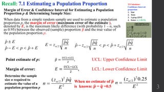
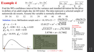
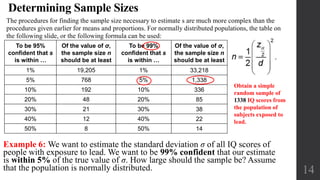
This document discusses estimating parameters and determining sample sizes from populations. It covers estimating population proportions, means, standard deviations, and variances. For each parameter, it describes how to construct confidence intervals and determine the necessary sample size. Formulas are provided for margin of error, t-scores, z-scores and the chi-square distribution, which is used for estimating variances and standard deviations. Examples show how to apply the concepts to find confidence intervals and critical values for specific population problems.

1. Elementary Statistics
Chapter 7:
Estimating Parameters
and Determining
Sample Sizes
7.3 Estimating a
Population Standard
Deviation or Variance
1

2. 7.1 Estimating a Population Proportion
7.2 Estimating a Population Mean
7.3 Estimating a Population Standard Deviation or Variance
7.4 Bootstrapping: Using Technology for Estimates
2
Chapter 7:
Estimating Parameters and Determining Sample Sizes
Objectives:
• Find the confidence interval for a proportion.
• Determine the minimum sample size for finding a confidence interval for a proportion.
• Find the confidence interval for the mean when  is known.
• Determine the minimum sample size for finding a confidence interval for the mean.
• Find the confidence interval for the mean when  is unknown.
• Find a confidence interval for a variance and a standard deviation.

3. Point estimate of p: 𝑝 =
𝑈𝐶𝐿+𝐿𝐶𝐿
2
, UCL: Upper Confidence Limit
Margin of error: 𝐸 =
𝑈𝐶𝐿−𝐿𝐶𝐿
2
, LCL: Lower Confidence Limit
Margin of Error & Confidence Interval for Estimating a Population
Proportion p & Determining Sample Size:
When data from a simple random sample are used to estimate a population
proportion p, the margin of error (maximum error of the estimate ),
denoted by E, is the maximum likely difference (with probability 1 – α, such
as 0.95) between the observed (sample) proportion 𝑝 and the true value of
the population proportion p.
3
ˆ
ˆ ˆ
p E
p E p p E

    2 2
ˆ ˆ ˆ ˆ
ˆ ˆ   
pq pq
p z p p z
n n
 
Recall: 7.1 Estimating a Population Proportion
2
ˆ ˆpq
E z
n

2
2
2
ˆ ˆ( )z pq
n
E


2
2
2
( ) 0.25z
n
E

When no estimate of 𝒑
is known: 𝒑 = 𝒒 =0.5
Determine the sample
size n required to
estimate the value of a
population proportion p
TI Calculator:
Confidence Interval:
proportion
1. Stat
2. Tests
3. 1-prop ZINT
4. Enter: x, n & CL

4. 4
Recall: 7.2 Estimating a Population Mean
Determine the sample size n required to estimate the
value of a population mean µ.
Confidence Interval for Estimating a Population Mean
2
2  
  
 
z
n
E
 
2 2
   
      
   
X z X z
n n
 
 

𝐶𝐼: 𝑥 ± 𝐸 →
2E z
n

 
  
 
2
s
E t
n

 
  
 
2 2
   
      
   
s s
X t X t
n n
 
Confidence Interval for Estimating a Population Mean with σ un Known
Point estimate of µ: 𝑥 =
𝑈𝐶𝐿+𝐿𝐶𝐿
2
, UCL: Upper Confidence Limit
Margin of error: 𝐸 =
𝑈𝐶𝐿−𝐿𝐶𝐿
2
,LCL: Lower Confidence Limit
σ Known
TI Calculator:
Z - interval
1. Stat
2. Tests
3. Z - Interval
4. Enter Data or Stats
5. Enter
TI Calculator:
T- Distribution: find the t-score
1. 2nd + VARS
2. invT(
3. 2 entries (Left Area,df)
4. Enter
TI Calculator:
T- interval
1. Stat
2. Tests
3. T - Interval
4. Enter Data or Stats
5. Enter

5. Key Concept:
Use sample standard deviation s (or a sample variance s²) to estimate the value
of the corresponding population standard deviation σ (or population variance σ²).
The sample variance s² is the best point estimate of the population variance σ².
To Construct a confidence interval estimate of a population standard deviation, use χ²
distribution.
When products that fit together (such as pipes) are manufactured, it is important to
keep the variations of the diameters of the products as small as possible; otherwise,
they will not fit together properly and will have to be scrapped.
In the manufacture of medicines, the variance and standard deviation of the medication
in the pills play an important role in making sure patients receive the proper dosage.
For these reasons, confidence intervals for variances and standard deviations are
necessary.
5
7.3 Estimating a Population Standard Deviation or Variance

6. Key points about the χ² (chi-square or chi-squared) distribution:
The chi-square distribution must be used to calculate confidence intervals for variances and standard deviations.
The chi-square variable is similar to the t variable in that its distribution is a family of curves based on the number of
degrees of freedom. The symbol for chi-square is χ² (Greek letter chi, pronounced “ki”).
A chi-square variable cannot be negative, and the distributions are skewed to the right.
At about 100 degrees of freedom, the chi-square distribution becomes somewhat symmetric.
The area under each chi-square distribution is equal to 1.00, or 100%.
In a normally distributed population with variance σ2 , assume that we
randomly select independent samples of size n and, for each sample,
compute the sample variance s2 (which is the square of the sample
standard deviation s).
The sample statistic χ2 (pronounced chi-square)
χ2 =
(𝑛−1)𝑠2
𝜎2 has a sampling distribution called the chi-square distribution.
6
7.3 Estimating a Population Standard Deviation or Variance, Chi-Square Distribution
2
2
2
( 1)n s





7. Chi-Square Distribution & Confidence Interval
Critical Values of χ² We denote a right-tailed critical value by χR
² and we denote a left-tailed
critical value by χL
². Those critical values can be found by using technology or χ² -Table.
Degrees of Freedom: df = n − 1
As the number of degrees of freedom increases, the chi-square distribution approaches a
normal distribution.
Not symmetric: Confidence interval estimate of σ² does not fit a format of
s² − E < σ² < s² + E, so we must do separate calculations for the upper and lower confidence
interval limits.
Critical value of χ² in the body of the table corresponds to an area given in the top row of the
table, and each area in that top row is a cumulative area to the right of the critical value.
7
2 2
2
2 2
right left
( 1) ( 1)
, d.f. = 1
n s n s
n
 
 
  
2 2
2 2
right left
( 1) ( 1)
, d.f. = 1
n s n s
n
 
 
  

8. Example 1: Finding Critical Value of 𝝌 𝟐
Find the values for χ²
R and χ²
L for a
90% confidence interval when n = 25.
8
df = n – 1 =24
χ²
R: 1 – 0.90 = 0.10.
Divide by 2 to get 𝐴 𝑅 = 0.05
χ²
L: 𝐴 𝐿 =1 – 0.05 = 0.95.
2 2
R L=36.415, =13.848 
TI Calculator
𝝌 𝟐
− Distribution Value
1. Math
2. Solver (at the bottom):
3. Put 𝝌 𝟐
CDF (2nd , Vars, Down
to 𝝌 𝟐
CDF): (Lower, Upper, df)
4. (Lower = 0, Upper = x, df),
Enter
5. Subtract
𝜶
𝟐
, and Enter
6. Click on Alpha key and Enter
Statistics calculator:
https://www.danielsoper.com/statcalc/default.aspx

9. Example 2: Finding Critical Value of χ²
Find the values for χ²
R and χ²
L for a 95%
confidence interval when n = 22.
9
2
R
2
L
=35.479
=10.283


df = n – 1 = 21
χ²
R: 1 – 0.95 = 0.05. Divide by 2 to get 𝐴 𝑅 = 0.025
χ²
L: 𝐴 𝐿 = 1 – 0.025 = 0.975

10. Confidence Interval for Estimating a Population Standard Deviation or Variance
σ = population standard deviation, σ² = population
variance
s = sample standard deviation, s² = sample variance
n = number of sample values
E = margin of error χ²
χ²
L = left-tailed critical value of χ²
χ²
R = left-tailed critical value of χ²
1. The sample is a simple random sample.
2. The population must have normally distributed
values. The requirement of a normal distribution is
much stricter here than in earlier sections, so large
departures from normal distributions can result in
large errors.
10
2 2
2
2 2
R L
( 1) ( 1)
d.f. = 1
n s n s
n

 
 
 

2 2
2 2
R L
( 1) ( 1)n s n s

 
 
 

11. Find the 95% confidence interval for the variance and standard deviation
of the nicotine content of cigarettes manufactured if a sample of 20
cigarettes has a standard deviation of 1.6 milligrams. (Assume ND)
Example 3
Solution: Given: Random sample and n = 20, s = 1.6 mg, 95% CI = ?
11
df = n – 1 = 19
χ²
R: 1 – 0.95 = 0.05 → 𝐴 𝑅 = 0.025
χ²
L: 𝐴 𝐿 =1 – 0.025 = 0.975
χ²
R = 32.852 and χ²
L = 8.907
2 2
2(19)(1.6) (19)(1.6)
32.852 8.907
 
2
1.4806 5.4609 
2 2
2
2 2
R L
( 1) ( 1)n s n s

 
 
 
2 2
2 2
R L
( 1) ( 1)n s n s

 
 
 
1.4806 5.4609
1.2168 2.3369


 
 

12. Find the 90% confidence interval for the variance and standard deviation for the price
in dollars of an adult single-day ski lift ticket. The data represent a selected sample of
nationwide ski resorts. Assume the variable is normally distributed.
59 54 53 52 51 39 49 46 49 48
Example 4
Solution: Given: ND Random sample and n = 10, 95% CI = ?
12
df = n – 1 = 9
χ²
R: 1 – 0.90 = 0.1 → 𝐴 𝑅 = 0.05
χ²
L: 𝐴 𝐿 = 1 – 0.05 = 0.95
χ²
R = 16.919, χ²
L = 3.325
2(9)(28.2) (9)(28.2)
16.919 3.325
 
2
15.0127 76.3910 
15.0127 76.3910
3.8746 8.7402


 
 
2 2
2
2 2
R L
( 1) ( 1)n s n s

 
 
 
2 2
2 2
R L
( 1) ( 1)n s n s

 
 
 
TI Calculator:
How to enter data:
1. Stat
2. Edit
3. ClrList 𝑳 𝟏
4. Or Highlight & Clear
5. Type in your data in
L1, ..
Mean, SD, 5-number
summary
1. Stat
2. Calc
3. Select 1 for 1 variable
4. Type: L1 (second 1)
5. Scroll down for 5-
number summary
Technology: s = 5.3125, s2 = 28.2

13. A group of 22 subjects took an IQ test during part of a study. The subjects
had a standard deviation IQ score of 14.3. Construct a 95% confidence
interval estimate of σ, the standard deviation of the population from which
the sample was obtained. (Assume Normally distributed data)
Example 5
Solution: Given: ND, Random sample and n = 22, s = 14.3, 95% CI = ?
13
Example 2: df = n – 1 = 21, s=14.3
χ²
R: 1 – 0.95 = 0.05 → 𝐴 𝑅 = 0.025
χ²
L: 𝐴 𝐿 = 1 – 0.025 = 0.975
2
R
2
L
=35.479
=10.283


2 2
222 1 14 3 22 1 14 3
35 479 10 283

 
 
( )( . ) ( )( . )
. .
2
121 0 417 6 . .
11 0 20 4 . .
Based on this result, we have 95% confidence that the
limits of 11.0 and 20.4 contain the true value of σ.
2 2
2
2 2
R L
( 1) ( 1)n s n s

 
 
 
2 2
2 2
R L
( 1) ( 1)n s n s

 
 
 

14. Determining Sample Sizes
The procedures for finding the sample size necessary to estimate s are much more complex than the
procedures given earlier for means and proportions. For normally distributed populations, the table on
the following slide, or the following formula can be used:
14
To be 95%
confident that s
is within …
Of the value of σ,
the sample size n
should be at least
1% 19,205
5% 768
10% 192
20% 48
30% 21
40% 12
50% 8
To be 99%
confident that s
is within …
Of the value of σ,
the sample size n
should be at least
1% 33,218
5% 1,338
10% 336
20% 85
30% 38
40% 22
50% 14
Example 6: We want to estimate the standard deviation σ of all IQ scores of
people with exposure to lead. We want to be 99% confident that our estimate
is within 5% of the true value of σ. How large should the sample be? Assume
that the population is normally distributed.
Obtain a simple
random sample of
1338 IQ scores from
the population of
subjects exposed to
lead.