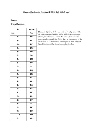
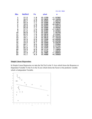
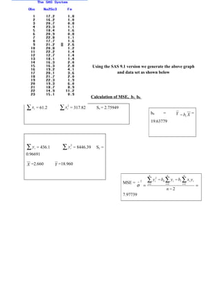
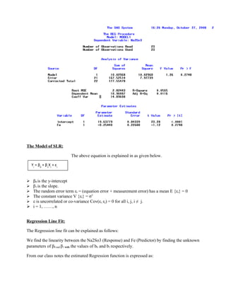
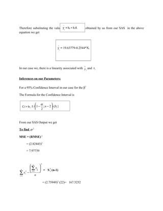
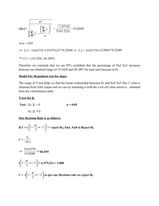
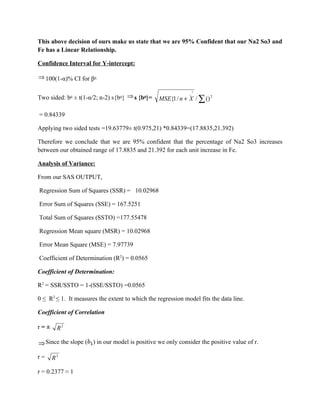
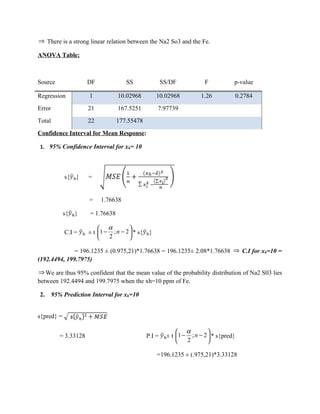
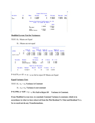
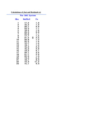
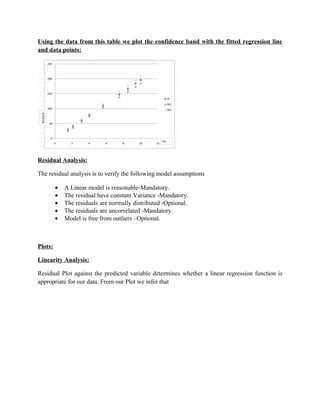
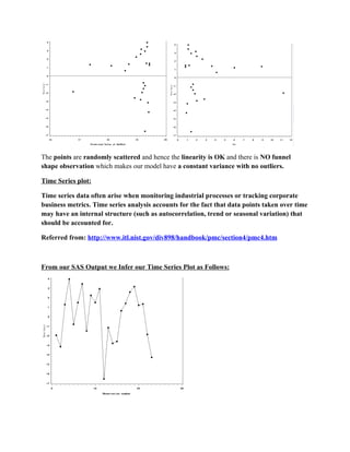
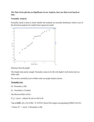
The document presents a linear regression analysis of sodium sulfite concentration (%w) and iron concentration (ppm) in waste water samples collected over 23 days. Key findings include: 1) A linear regression model was fit relating sodium sulfite to iron. 2) Statistical tests showed the relationship between the two variables was statistically significant. 3) Residual analysis confirmed assumptions of linearity, normality and constant variance were met.

1. Advanced Engineering Statistics-IE 5318- Fall 2008-Project1
Report:
Project Proposal:
Fe Na2SO3
The main objective of this project is to develop a model for
ppm %w
the concentration of sodium sulfite with the concentration
1.8 17.2 of Iron present in waste water. We have collected waste
water samples on each day for 23 days so our number of the
1.0 16.2
observation is 23. Performed lab analysis (ICP) to find out
0.8 20.7 Fe and Sodium sulfite from plant production data.
1.1 23.3
1.6 18.4
0.8 20.9
1.1 22.8
1.6 17.7
2.6 21.2
1.2 20.8
1.4 22.2
1.4 12.7
1.4 18.1
2.0 16.3
2.8 16.3
4.1 19.2
3.6 20.1
2.0 21.7
1.9 22.3
6.0 19.3
8.9 18.7
11.2 14.9
0.9 15.1

2. Calculations of yhat and Residuals (e)

3. Simple Linear Regression:
In Simple Linear Regression we take the Na2 So3 in the Y-Axis which forms the Response or
Dependent Variable Vs the Fe in the X-axis which forms the Factor or the predictor variable
which is Independent Variable.

4. Using the SAS 9.1 version we generate the above graph
and data set as shown below
Calculation of MSE, b1, b0.
∑x i = 61.2 ∑x 2
i = 317.82 Sx = 2.75949
b0 = Y − b1 X =
19.63779
∑y i = 436.1 ∑y 2
i = 8446.39 Sy =
0.96691
X =2.660 Y =18.960
n n n
MSE = ∧ 2 ∑y 2
i − b0 ∑ y i − b1 ∑ xi y i
σ = i =1 i =1 i =1
=
n−2
7.97739

5. The Model of SLR:
The above equation is explained in as given below.
Yi = β0 + β1Xi + εi
 β0 is the y-intercept
 β1 is the slope.
 The random error term εi = (equation error + measurement error) has a mean E {εi} = 0
 The constant variance V {εi} = σ2
 ε is uncorrelated or co-variance Cov(εi, εj) = 0 for all i, j, i ≠ j.
 i = 1, ……, n
Regression Line Fit:
The Regression line fit can be explained as follows:
We find the linearity between the Na2So3 (Response) and Fe (Predictor) by finding the unknown
parameters of β0 and β1 with the values of b0 and b1 respectively.
From our class notes the estimated Regression function is expressed as:

6. ^
Therefore substituting the valuesYof bb0+andi b1
i
= 0 b1X obtained by us from our SAS in the above
equation we get
^
Yi = 19.63779-0.2544*Xi
∧
In our case we, there is a linearity associated with y i and xi
Inferences on our Parameters:
For a 95% Confidence Interval in our case for the β1
The Formula for the Confidence Interval is
 α 
C.I = b1 ± t 1 − ; n − 2  s{b1 }
 2 
From our SAS Output we get
To find σ 2
MSE = (RMSE) 2
= (2.82443)2
= 7.97739
2
 n 
∑ x  2
 i =1 i  = S x (n-1)
n
∑ xi − n
i =1
2
= (2.75949)2 (22)= 167.5252

7. σ2
2
 n  7.97739
s{b1}=  ∑ xi  = = 0.22688
n 167.5252
∑ xi −  i =1n 
i =1
2
At α = 0.05
⇒ C.I = 19.63779 ± t ( 0.975,21) * 0.22688 ⇒ C.I = 19.63779 ± (2.080) * 0.22688
⇒ C.I = (19.1658, 20.1097)
Therefore we conclude that we are 95% confident that the percentage of Na2 So3 increases
between our obtained range of 19.1658 and 20.1097 for each unit increase in Fe.
Model Fit: Hypothesis test for slope:
The usage of T-test helps us find the linear relationship between Fe and Na2 So3.The t* value is
obtained from SAS output and we can try matching it with the t-cut off value which is obtained
from the t-distribution table.
T-test for β1
Test: H0: β1 = 0 α = 0.05
H1: β1 ≠ 0
Our Decision Rule is as follows:
 α 
If t* > t 1 − ; n − 2  → reject H0; Else, Fail to Reject H0
 2 
b1
t* =
s{b1 }
19.63779
⇒ ⇒ 86.555
0.22688
 α 
t 1 − ; n − 2  = t(.975,21) = 2.080
 2 
 α 
t* > t 1 − ; n − 2  As per our Decision rule we reject H0
 2 

8. This above decision of ours make us state that we are 95% Confident that our Na2 So3 and
Fe has a Linear Relationship.
Confidence Interval for Y-intercept:
⇒ 100(1-α)% CI for β0.
_2
Two sided: b0 ± t(1-α/2; n-2) s{b0} ⇒ s {b0}= MSE{1 / n + X / ∑ () 2
= 0.84339
Applying two sided tests =19.63779± t(0.975,21) *0.84339=(17.8835,21.392)
Therefore we conclude that we are 95% confident that the percentage of Na2 So3 increases
between our obtained range of 17.8835 and 21.392 for each unit increase in Fe.
Analysis of Variance:
From our SAS OUTPUT,
Regression Sum of Squares (SSR) = 10.02968
Error Sum of Squares (SSE) = 167.5251
Total Sum of Squares (SSTO) =177.55478
Regression Mean square (MSR) = 10.02968
Error Mean Square (MSE) = 7.97739
Coefficient of Determination (R2) = 0.0565
Coefficient of Determination:
R2 = SSR/SSTO = 1-(SSE/SSTO) =0.0565
0 ≤ R2 ≤ 1. It measures the extent to which the regression model fits the data line.
Coefficient of Correlation
r=± R2
Since the slope ( ) in our model is positive we only consider the positive value of r.
r= R2
r = 0.2377 ≈ 1

9. ⇒ There is a strong linear relation between the Na2 So3 and the Fe.
ANOVA Table:
Source DF SS SS/DF F p-value
Regression 1 10.02968 10.02968 1.26 0.2784
Error 21 167.5251 7.97739
Total 22 177.55478
Confidence Interval for Mean Response:
1. 95% Confidence Interval for xh= 10
s{ } =
= 1.76638
s{ } = 1.76638
 α 
C.I = ± t 1 − ; n − 2  * s{ }
 2 
= 196.1235 ± (0.975,21)*1.76638 = 196.1235± 2.08*1.76638 ⇒ C.I for xh=10 =
(192.4494, 199.7975)
⇒ We are thus 95% confident that the mean value of the probability distribution of Na2 S03 lies
between 192.4494 and 199.7975 when the xh=10 ppm of Fe.
2. 95% Prediction Interval for xh=10
s{pred} =
 α 
= 3.33128 P.I = ± t 1 − ; n − 2  * s{pred}
 2 
=196.1235 ± (.975,21)*3.33128

10. =196.1235 ± 6.929 ⇒ P.I for xh =10 =
(189.1945, 203.0525)
⇒ We predict with 95% confidence that the actual ppm of Fe obtained when the xh=10 ppm of
Fe lies between 189.1235 and 203.0525.
3. 95% Confidence Band for xh= 10
± w s{ }
Where = 2F (1-α/2,2,n-2)
=2*F (0.95, 2, 21)
=2*19.425
= 38.85
= 6.2329~6.233
C.B = 196.1235 ± 6.233*1.76638
= 196.1235 ± 11.0098
=(185.1137,207.1333)
⇒ C.B for xh=10 = (185.1137, 207.1333)
⇒ We have 95% confidence that true regression line lies certainly between the upper and
lower band of the CB. So for xh=10 of Fe obtained will lie between 185.1137 and 207.1333
From the above results we infer that CB is wider than CI
= > = , which is always true. The Confidence
Band limits for several xh along the range of x:

11. Using the data from this table we plot the confidence band with the fitted regression line
and data points:
Residual Analysis:
The residual analysis is to verify the following model assumptions
• A Linear model is reasonable-Mandatory.
• The residual have constant Variance -Mandatory.
• The residuals are normally distributed -Optional.
• The residuals are uncorrelated -Mandatory.
• Model is free from outliers –Optional.
Plots:
Linearity Analysis:
Residual Plot against the predicted variable determines whether a linear regression function is
appropriate for our data. From our Plot we infer that

12. The points are randomly scattered and hence the linearity is OK and there is NO funnel
shape observation which makes our model have a constant variance with no outliers.
Time Series plot:
Time series data often arise when monitoring industrial processes or tracking corporate
business metrics. Time series analysis accounts for the fact that data points taken over time
may have an internal structure (such as autocorrelation, trend or seasonal variation) that
should be accounted for.
Referred from: http://www.itl.nist.gov/div898/handbook/pmc/section4/pmc4.htm
From our SAS Output we Infer our Time Series Plot as Follows:

13. The Time Series plot has no Significance in our Analysis, since our data is not based on
time.
Normality Analysis:
Normality check is done to check whether the residuals are normally distributed, which is one of
the desired assumption for simple linear regression model
.
Inference from the graph:
The Graph looks pretty straight. Normality seems to be Ok with slight S with shorter tails on
either ends.
We can do a normality test to further make our graph analysis clearer.
Normality test:
H0 : Normality is OK
H1 : Normality is Violated.
Our Decision Rule will be :
If < c(α,n) → Reject H0 else we fail to H0
Take α=0.05; c(0.1,23)=0.964 =0.97415 (from SAS output corresponding ENRM VALUE)
⇒ Since > c(α,n) ⇒ Normality is OK.

14. Modified Levene Test for Variances:
TEST: H0 : Means are Equal
H1 : Means are not equal
P=0.6576, α=.05 ⇒ P > α we fail to reject H0 Means are Equal
Equal Variance Test:
TEST: H0 : σd1 = σd2 Variance is Constant
H1 : σd1 ≠ σd2 Variance is not constant
P=0.1990; α= 0.05 ⇒ P > α We Fail to Reject H0 Variance is Constant.
From Modified Levene test, we conclude Constant Variance is constant, which is in
accordance to what we have observed from the Plot Residual Vs Yhat and Residual Vs x.
So we need not do any Transformations.

15. Conclusion:
From all the above tests performed we conclude the following:
There is a linear relation between the Na2So3(Response) and Fe(Predictor).
The fitted regression line in our model is represented by the equation:
^
Y = 19.637739 -0.2544 x
i
The T-test further proves that there is a linear regression to relate Na2So3 to Fe. The R value (
=0.0565) in our model indicates that there is a good fit and it explains everything in estimating
the Na2 So3 considering the Fe as the predictor variable.
We took the significance level as α=0.05 to conduct all our tests and our confidence level is
95% for all conclusions.
We calculated the Confidence intervals for the intercept of the regression function and also we
calculated the Confidence interval, Prediction interval and Confidence band for a given
value of ( =10). From the above mentioned calculations, we found that the prediction interval
is wider than the Confidence Interval for the same Confidence level of 95%.We also found that
the Confidence band is wider than the Confidence Interval.
We did Calculate the ANOVA table and found the Degrees of freedom and their corresponding
SSR,SSE,SSTO, MSR,MSE, F*,P-value which gave us the relationship between the Na2So3
and Fe.
We also did find out that the Variances of the error terms were normal and constant and also did
the residual analysis and found that the linearity was Ok with no funnel shape which attributed to
the constant variance. This was further supported by Modified Levene Test which states that
there is a constant Variance with equal means.
We also performed the Normality Test and found out that the Normality is Ok and the plot
suggested that the normality seems to be Ok with slight S with shorter tails on either ends and
got supported with the Normality Test. The plot between the residual and the normal scores
appeared pretty linear.