Downloaded 175 times
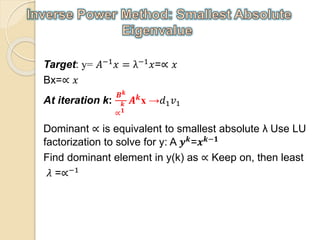
![Target: y=A 𝐱=𝜆𝐱
Start with all 1’s x vector: 𝒙 𝟎
=[1,1,……1] 𝑻
𝑦(1)=A𝑥(0)=λ(1) 𝑥(1) (Iteration number = 1)
λ(1)
= element in 𝑦1with highest absolute value
𝑥(1)
=
1
λ(1) 𝑦(1)
=
1
λ(1) A𝑥(0)
,
𝑦(2)
=A𝑥(1)
=
1
λ(1) 𝐴2
𝑥(0)
(Iteration number = 2)
λ(2)
= element in 𝑦2with highest absolute value
𝑥(2)
=
1
λ(2) 𝑦(2)
=
1
λ1λ2
𝐴2
𝑥(0)
………..
𝒚(𝒌)=A𝒙(𝒌−𝟏) → 𝒙(𝒌)=
𝟏
𝝀(𝒌) 𝒚(𝒌)→𝒙(𝒌) ≈
𝟏
𝝀(𝒌) 𝑨 𝒌 𝒙(𝟎)](https://image.slidesharecdn.com/powermethod-151224174633/85/Power-method-9-320.jpg)
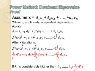
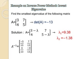
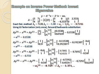
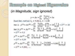


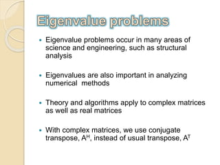
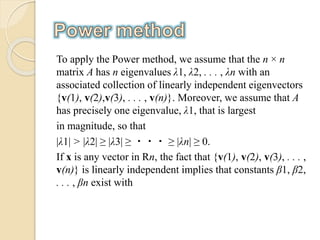
The document discusses eigenvalue problems and algorithms for solving them. Eigenvalue problems involve finding the eigenvalues and eigenvectors of a matrix and occur across science and engineering. The properties of the eigenvalue problem, like whether the matrix is real or complex, affect the choice of algorithm. The Power Method is described as an iterative technique for determining the dominant eigenvalue and eigenvector of a matrix. It works by successively applying the matrix to a starting vector to isolate the component in the direction of the dominant eigenvector. Variants can find other eigenvalues like the smallest. General projection methods approximate eigenvectors within a subspace, while subspace iteration generalizes Power Method to compute multiple eigenvalues.