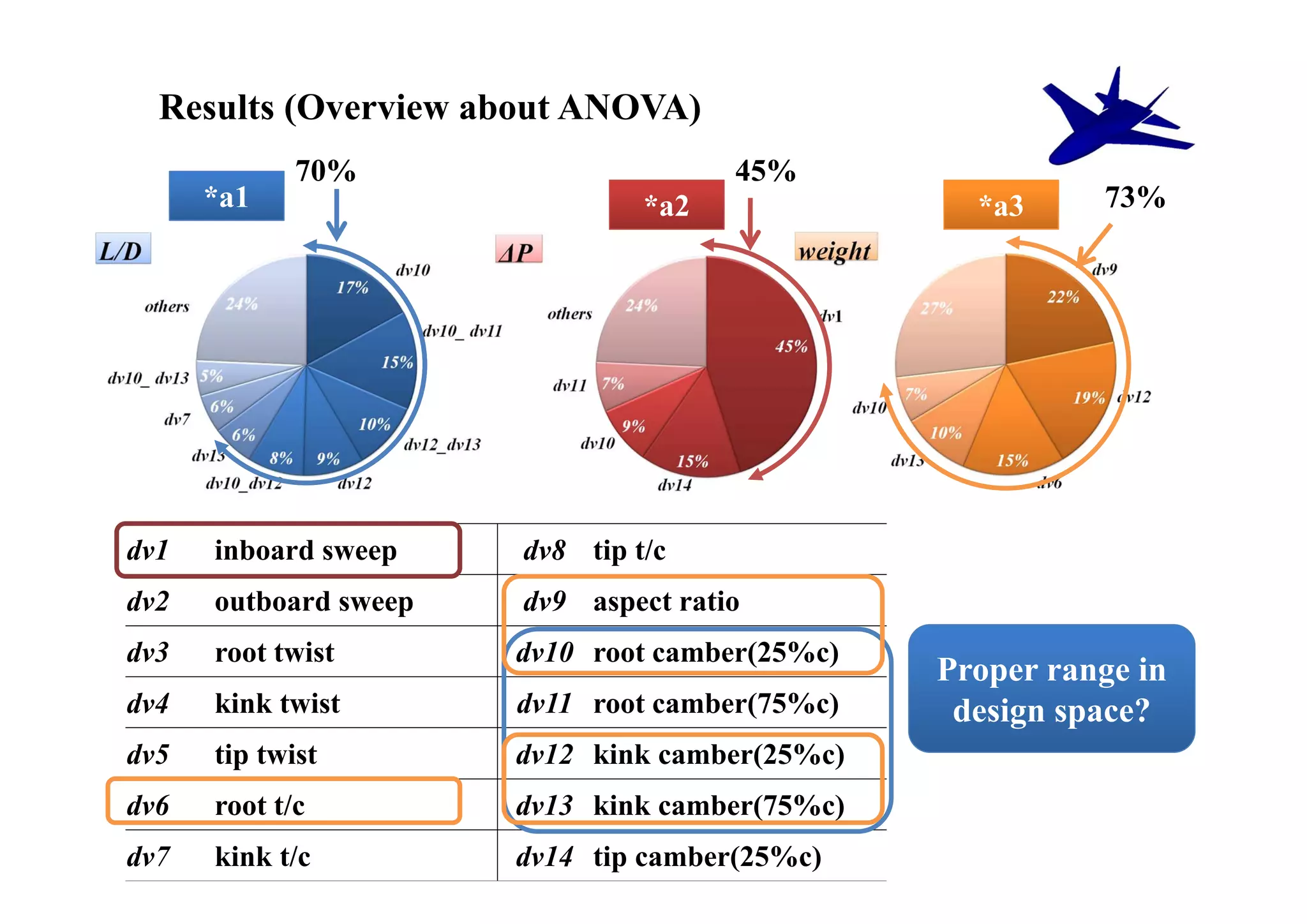
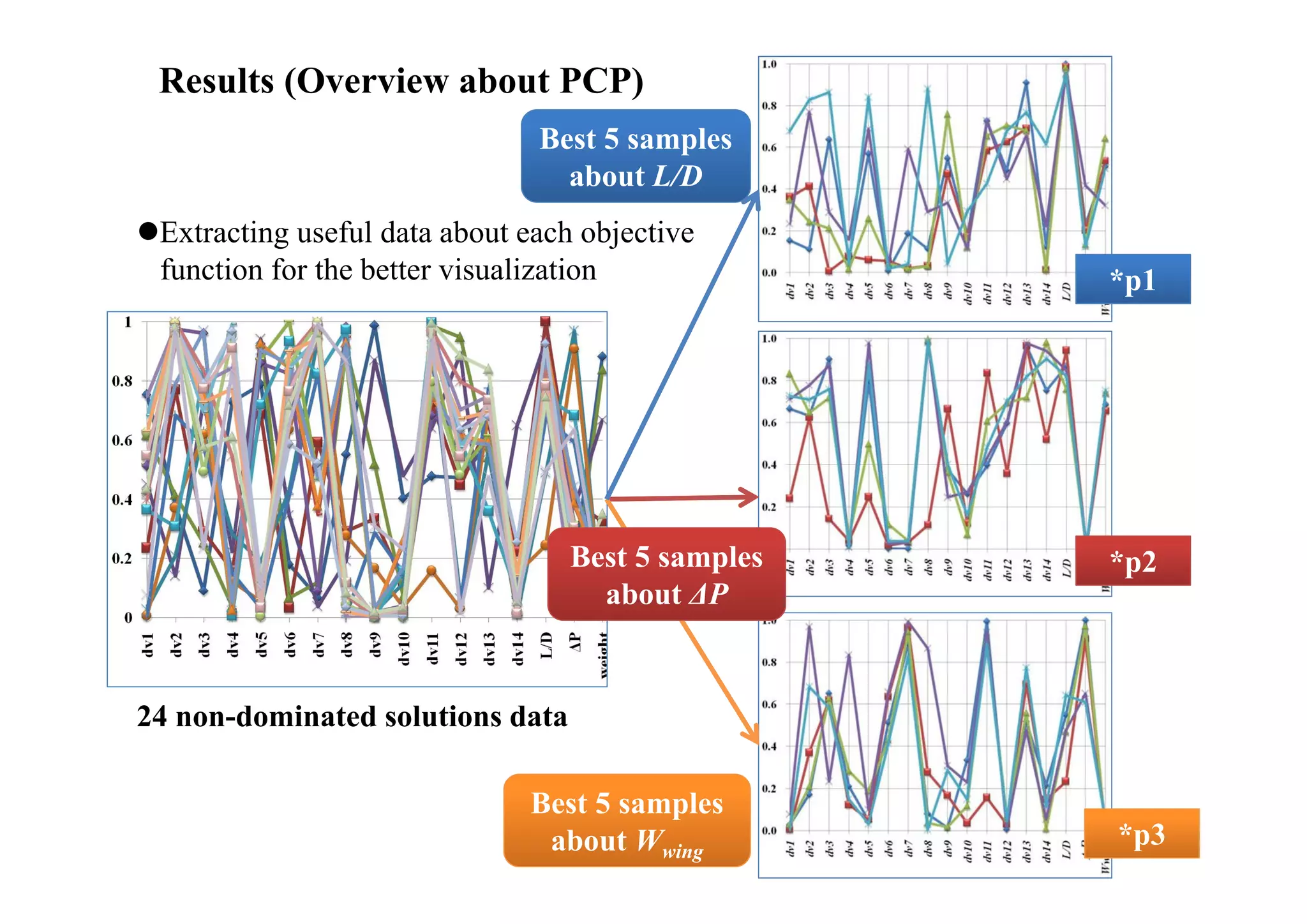
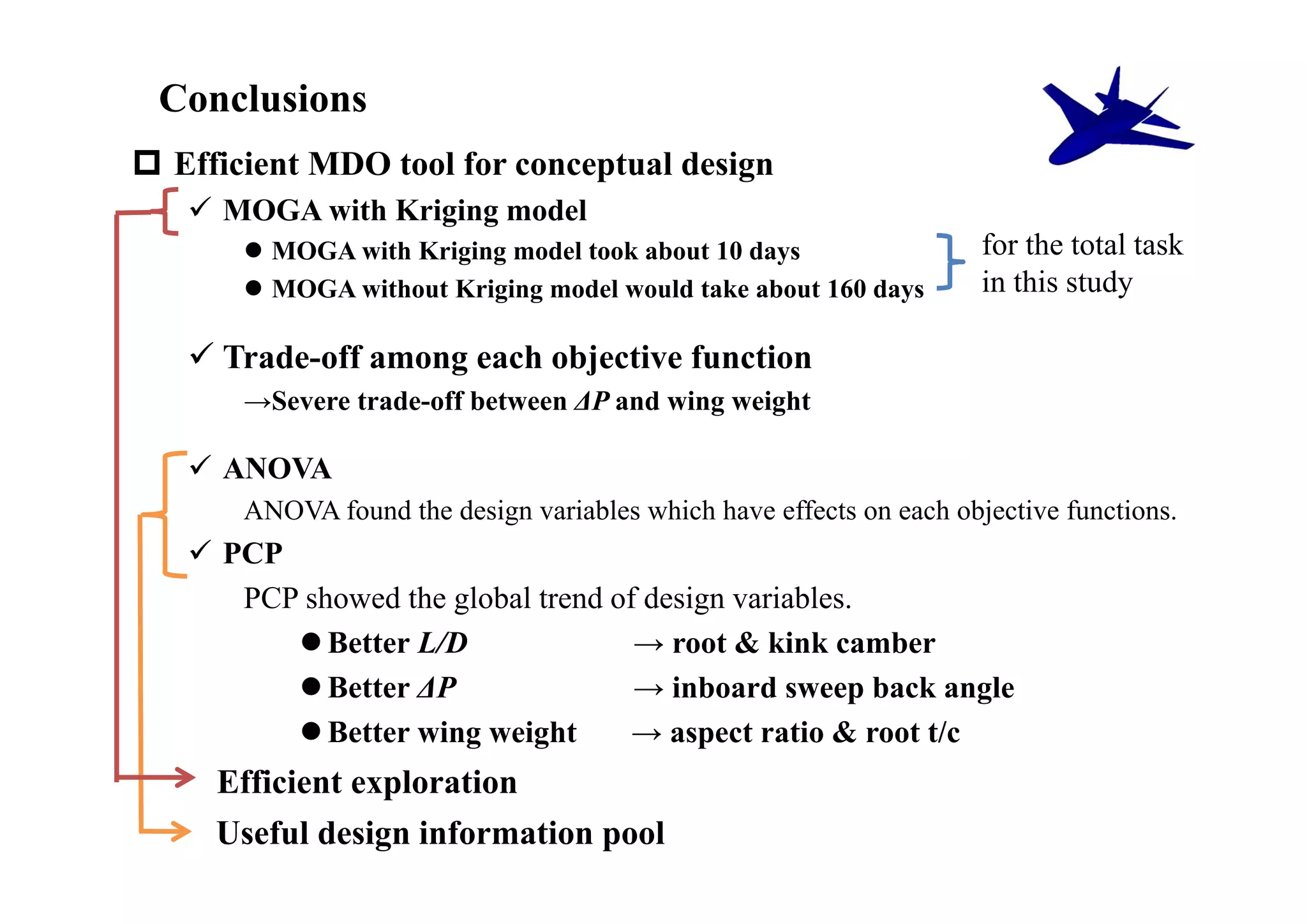
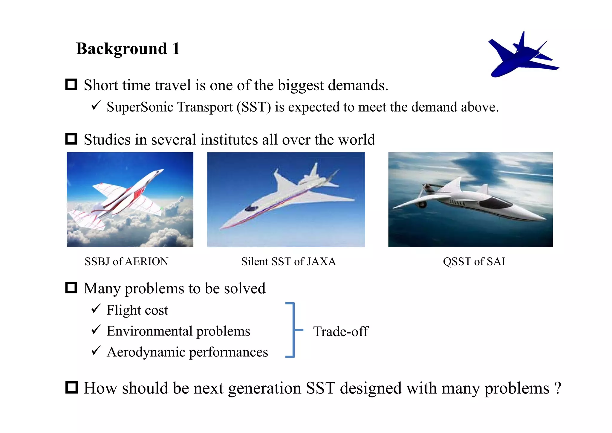
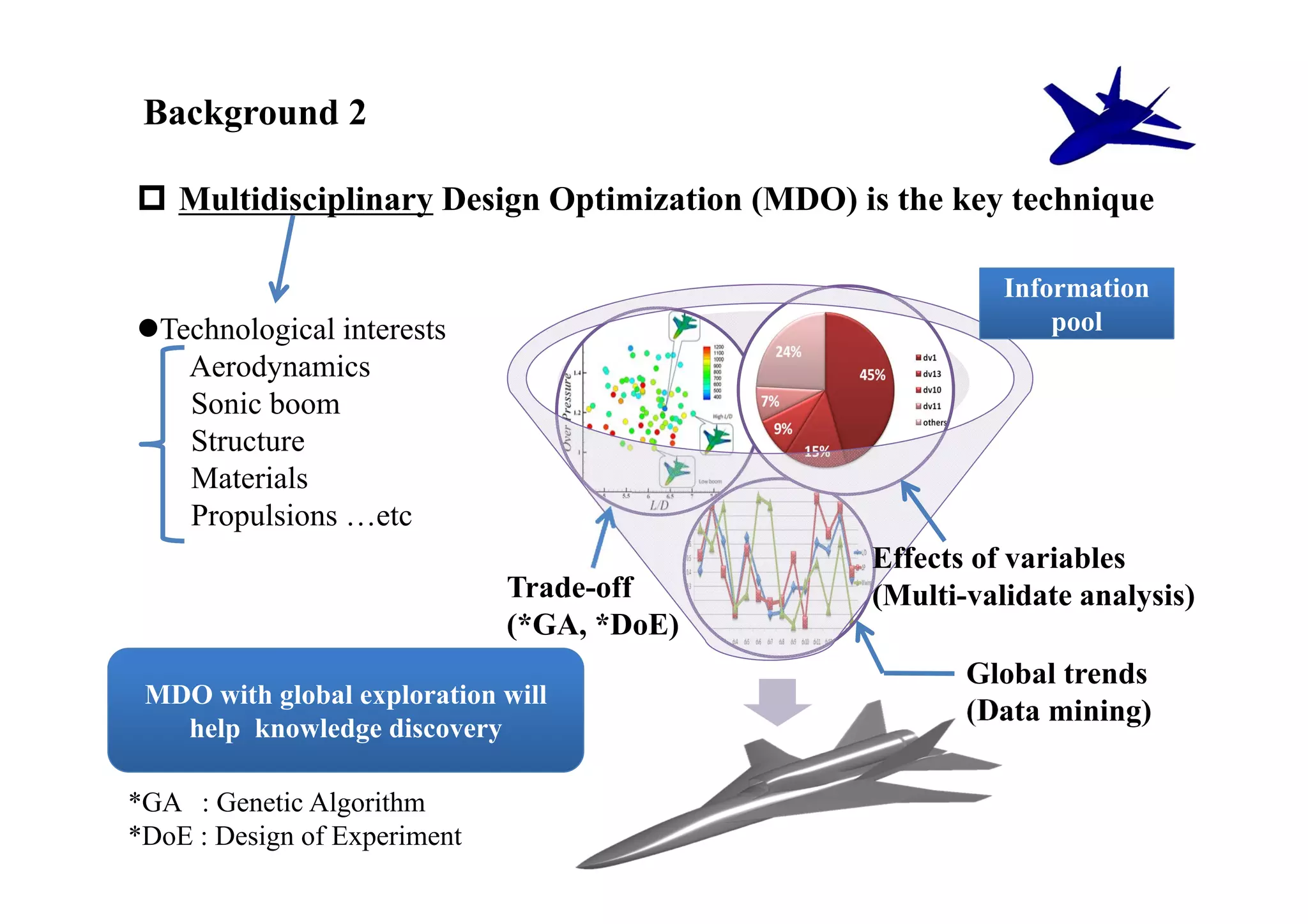
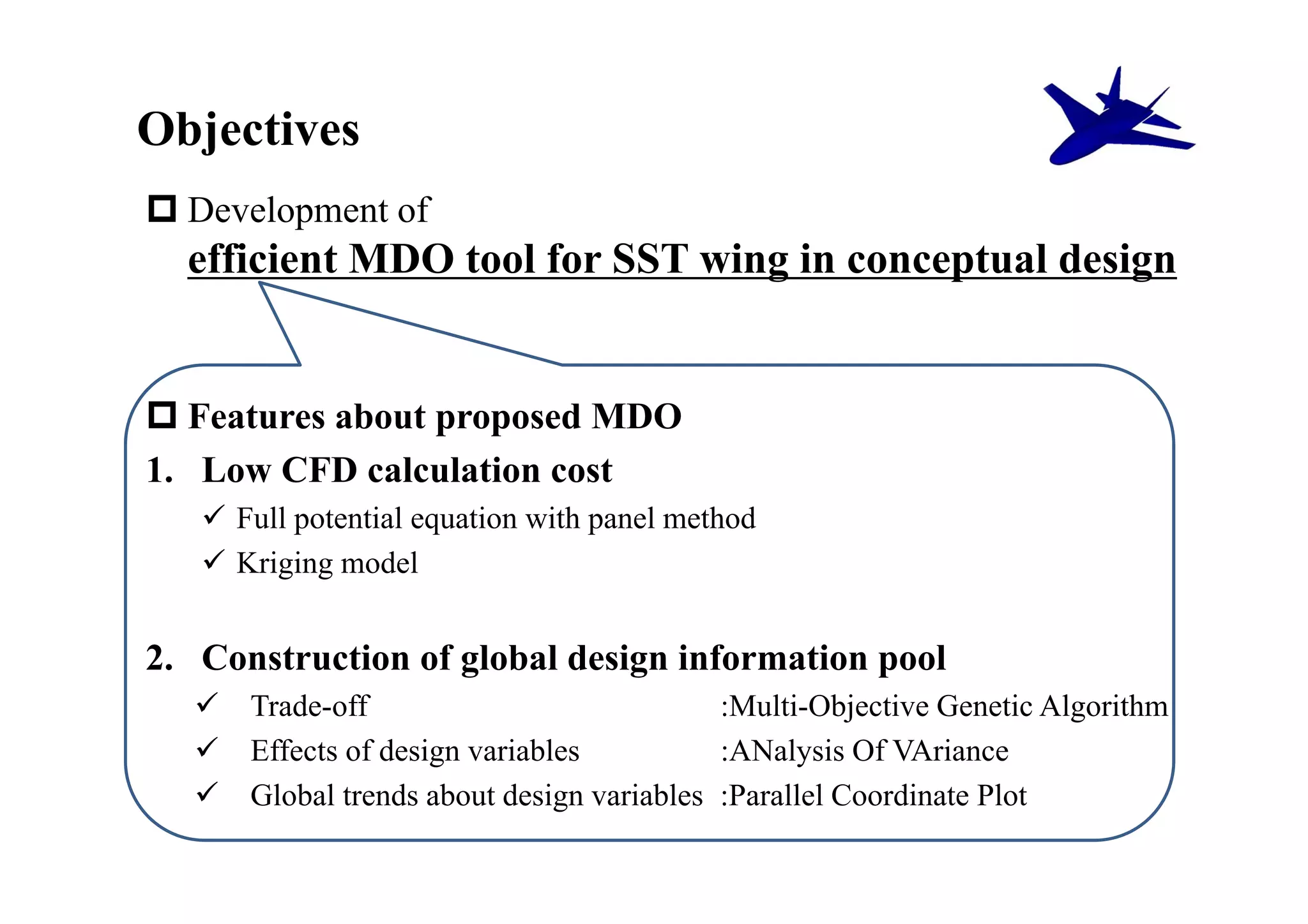
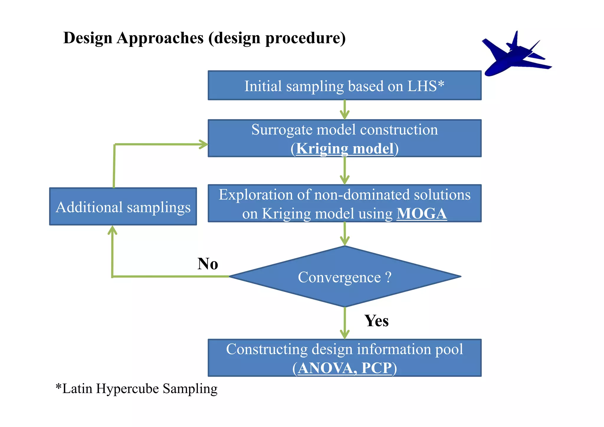
The document summarizes research on the multidisciplinary design optimization of supersonic transport wing concepts. The objectives were to develop an efficient MDO tool for conceptual design of SST wings using low-cost computational fluid dynamics and surrogate modeling. 107 design samples were evaluated for aerodynamic performance, sonic boom levels, and wing weight. 24 non-dominated solutions were identified, with the best designs having thinner root airfoils, larger inboard sweep angles, or modified tail angles compared to a baseline compromised design. Analysis of variance identified key design variables with the most influence on objectives.

1. 27th ICAS at Nice on 22th September
Session : Supersonic Aircraft Concepts
“Multidisciplinary Design Optimization of Supersonic Transport Wing
Using Surrogate Model”
Naoto Seto (Tokyo Metropolitan University)

2. Outline
 Background
 Objectives
 Design Approaches
 Design Target and Design Variables
 Objective Functions and Constraints
 Results
 Conclusions

3. Background 1
 Short time travel is one of the biggest demands.
 SuperSonic Transport (SST) is expected to meet the demand above.
 Studies in several institutes all over the world
SSBJ of AERION Silent SST of JAXA QSST of SAI
 Many problems to be solved
 Flight cost
 Environmental problems Trade-off
 Aerodynamic performances
 How should be next generation SST designed with many problems ?

4. Background 2
 Multidisciplinary Design Optimization (MDO) is the key technique
Information
Technological interests pool
Aerodynamics
Sonic boom
Structure
Materials
Propulsions …etc
Effects of variables
Trade-off (Multi-validate analysis)
(*GA, *DoE)
Global trends
MDO with global exploration will
(Data mining)
help knowledge discovery
*GA : Genetic Algorithm
*DoE : Design of Experiment

5. Objectives
 Development of
efficient MDO tool for SST wing in conceptual design
 Features about proposed MDO
1. Low CFD calculation cost
 Full potential equation with panel method
 Kriging model
2. Construction of global design information pool
 Trade-off :Multi-Objective Genetic Algorithm
 Effects of design variables :ANalysis Of VAriance
 Global trends about design variables :Parallel Coordinate Plot

6. Design Approaches

7. Design Approaches (design procedure)
Initial sampling based on LHS*
Surrogate model construction
(Kriging model)
Exploration of non-dominated solutions
Additional samplings on Kriging model using MOGA
No
Convergence ?
Yes
Constructing design information pool
(ANOVA, PCP)
*Latin Hypercube Sampling

8. Design Approaches (exploration of non-dominated solutions)
 Multi Objective Genetic Algorithm (MOGA)
 One of evolutionary algorithm
 Searching global non-dominated solutions with multi-point explorations
→Many evaluations are required.
CFD
Kriging model
One of surrogate model
Interpolating and searching local extremes
ˆ (x i )     (x i )
y
Global model Localized deviation
from the global model

9. Design Approaches (exploration of non-dominated solutions)
 Kriging model includes uncertainty at the predicted points.
 Expected Improvement (EI) considers the balance between optimist and the error.
 EI is expressed below (for maximization problem)
E I x  
z
 ( f max  z ) dz ,
n ：standard distribution,
 normal density
s ：standard error
 f  ˆ 
y  f max  ˆ 
y
 ( f max  y
ˆ )   max   s  
 s   s 
: Kriging model : Maximum values from sampling
 The larger EI value has the larger possibility to be optimum solutions
→Additional samplings are based on EIs’ maximization
Jones, D. R., “Efficient Global Optimization of
Expensive Black-Box Functions,” J. Glob.
Opt., Vol. 13, pp.455-492 1998.

10. Design Approaches (design information)
 Analysis of Variance (ANOVA)
 One of multi-validate analysis for quantitative information
Integrate
The main effect of design variable xi:
i ( xi )     y( x1 ,....., xn )dx1 ,..., dxi 1 , dxi 1 ,.., dxn  
ˆ
variance
where:
     y( x1 ,....., xn )dx1 ,....., dxn
ˆ
Total proportion to the total variance:
pi  
2
p2
 y(x1,....,xn ) dx1...dxn
35%
ˆ
p1
where, ε is the variance due to design variable xi. 65%
Main effect

11. Design Approaches (design information)
 Parallel Coordinate Plot (PCP)
 One of statistical visualization techniques from high-dimensional data into
two dimensional data.
 Design variables and objective functions are set parallel in the normalized axis.
 PCP shows global trends of design variables.
1.0
0.8
0.6
0.4
0.2
0.0
Upper bound of ith design variables
and objective functions Normalization
Lower bound of ith design variables x(dvi ) - min(dvi )
P
i
and objective functions max(dvi ) - min(dvi )

12. Design Target and Design Variables

13. Design Target
 Three-dimensional geometry of supersonic main wing
 Other components geometry fuselage, tail planform are same as
2.5th Silent SuperSonic Technology Demonstrator (S3TD)
Specifications
Fuselage 13.8m
MTOW 3500kg
Sref 21m2
Cruse M 1.6
Cruse altitude 14km
2.5th design by JAXA

14. Design Variables
 14 design variables Table 1 Design space
Upper Lower
Design variable
bound bound
Sweepback angle at inboard
dv1 57 (°) 69 (°)
section
Sweepback angle at outboard
dv2 40 (°) 50 (°)
section
dv3 Twist angle at wing root 0 (°) 2(°)
dv4 Twist angle at wing kink –1 (°) 0 (°)
dv5 Twist angle at wing tip –2 (°) –1 (°)
dv6 Maximum thickness at wing root 3%c 5%c
Root & kink airfoil NACA 64series dv7 Maximum thickness at wing kink 3%c 5%c
Tip airfoil bi-convex
dv8 Maximum thickness at wing tip 3%c 5%c
dv9 Aspect ratio 2 3
Tip airfoil
Supersonic- dv10 Wing root camber at 25%c –1%c 2%c
linearly-interpolation
leading edge dv11 Wing root camber at 75%c –2%c 1%c
Kink airfoil dv12 Wing kink camber at 25%c –1%c 2%c
spline-interpolation Subsonic- dv13 Wing kink camber at 25%c –2%c 1%c
leading edge dv14 Wing tip camber at 25%c –2%c 2%c
Root airfoil

15. Objective Functions and Constraints

16. Objective Functions
 Three objective functions in this study
maximize L/ D
minimize ΔP (On boom carpet)
ΔP
minimize Wwing
subject to Design C L = 0.105
Time[ms]
maximize
K-means method
ˆ - L / Dmax
y ˆ - L / Dmax
y
• EIL / D = ( ˆ - L / Dmax )Φ(
y ) + sφ( ) Additional sampling points
s s
maximize
clusters
ΔP - ˆ y ΔP - ˆ y
EI1
• EIΔP = ( ΔP - y
min
ˆ )Φ( min ) + sφ( min )
s s
maximize
Wwingmin ˆy Wwingmin - ˆ
y EI2
• EIWwing = (Wwingmin - ˆ )Φ(
y ) + sφ( )
s s

17. Evaluations of L/D and ΔP
 CAPAS* developed in JAXA
 Aerodynamic performance  Sonic-boom intensity
 Compressible potential equation  Correction of shock wave
with panel method (PANAIR) by Whitham’s theory
 2  2  2  PANAIR data
2 F ( x)  CP
( M  1) 2
 2
 2
0 2
x y z
x  
  1 r F x 
 ： Velocity potential
2 3
Thomas’s waveform parameter
method
  M 2－1
pressure[psf]
  1.4
Computational CP distributions r : propagation distance
geometry
Time[ms]
*CAPAS (CAD-based Automatic Panel Analysis System)

18. Evaluation of wing weight
 Inboard wing (multi-frame structure)
 Aluminum material
 Minimum thickness of skin & frame (0<thickness<20mm, every0.1mm)
 Outboard wing (full-depth honeycomb sandwich structure)
 Composite material
 Stack sequence
 Fiber angle θ ; [0/ θ/- θ/90] ns, θ=15, 30, 45, 60, 70deg
 Number of laminations n  n  N  25
 Solver is MSC NASTRAN 2005R (FEM model)
 Strength requirements
 Aluminum material：Mises stress < 200MPa at all FEM nodes
 Composite material: Destruction criteria < 1 at all FEM nodes on each laminate
 Computational conditions
 Symmetrical maneuver +6G, Safety rate: 1.25 PANAIR data
 Estimated load on the main wing
(symmetrical maneuver) × (safety rate) × (aerodynamics load)

19. Constraint
 Trim balance
C. G.
 C.P. is identical to C.G. at target CL
C.P.
→12 evaluations are required to decide
the angle of horizontal tail.
 Realistic cruise condition Angle of horizontal tail
 Blue area (main wing and horizontal tail)
were changed in this study.
Cl
target CL
Cd
x

20. Results

21. Results (samplings)
 75 points were sampled for constructing a initial Kriging model.
 Additional samplings were carried out three times.
 32 additional samples
 Total number of samplings is 107.
 Calculation time for one sample
 One hour for the CAPAS evaluations
 15 minutes for the NASTRAN evaluations
 Calculation environment
 General work station : 1CPU (Xeon 2.66MHz)

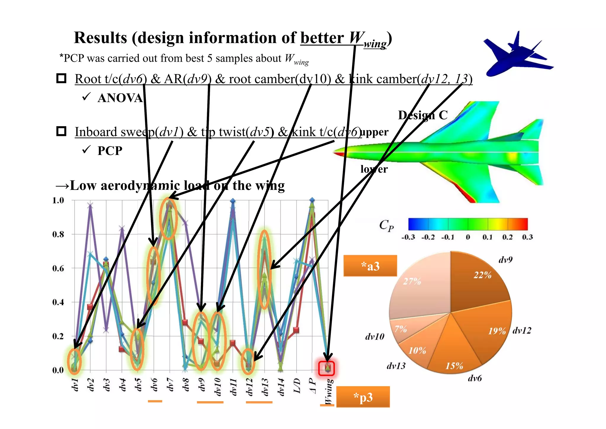
22. Results (solution space about objective functions)
Wwing
 24 non-dominated solutions from L/D ΔP[psf] AoA
[kg]
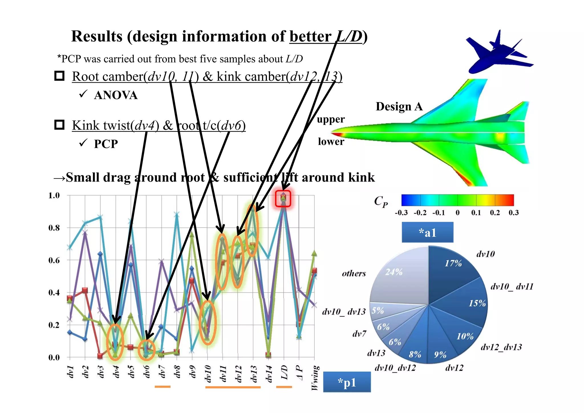
final data Design A 7.02 1.19 612 2.5
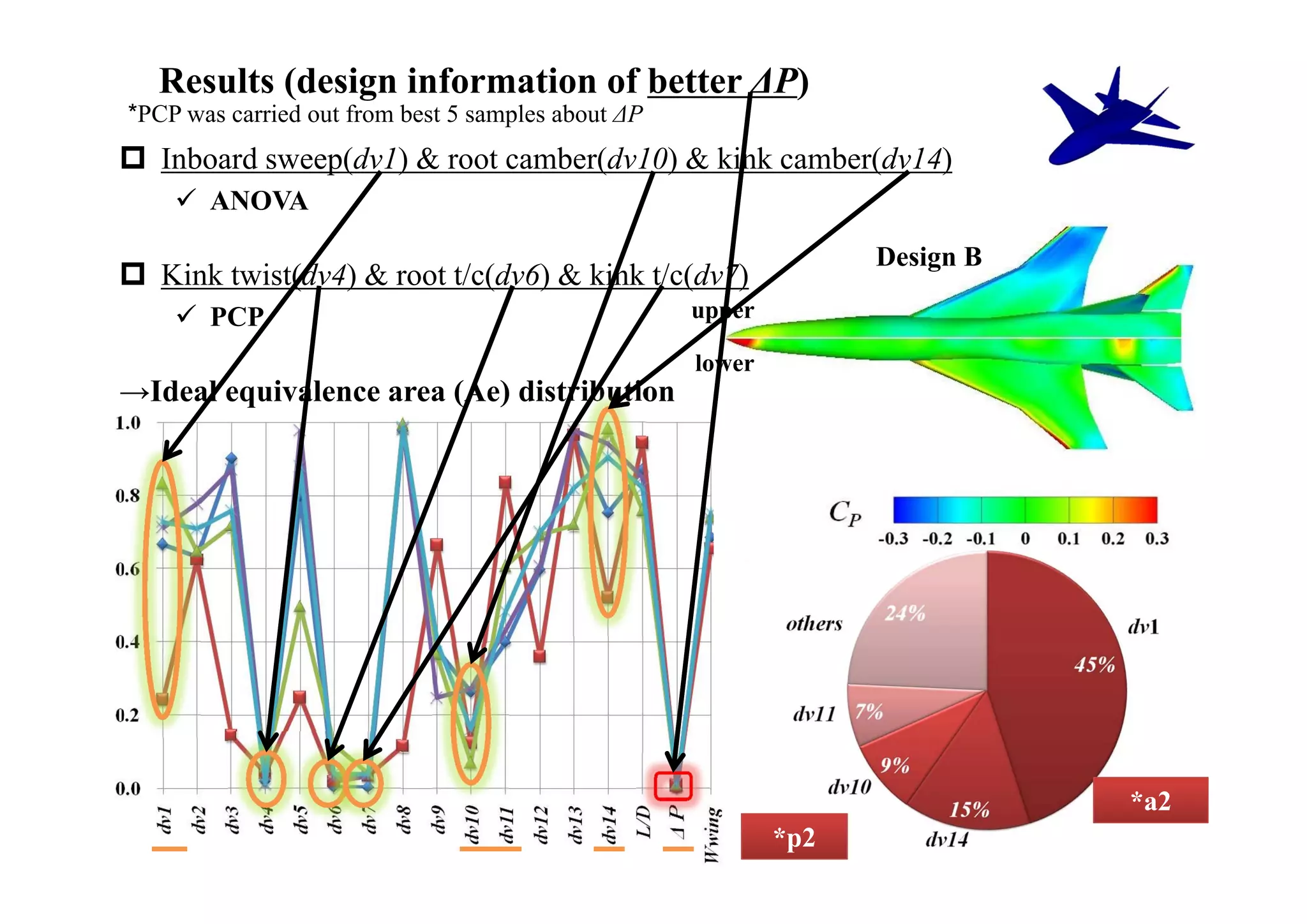
 Most of additional samplings formed Design B 6.08 0.97 502 2.7
non-dominated solutions Design C 5.60 1.53 276 2.6
Design D 6.77 1.09 691 2.6
Design A (best L/D) Design B (best ΔP) Design C (best Wwing)
Design D (compromised)
Wwing[kg]
ΔP[psf]
Optimum direction
L/D ΔP[psf]

23. Results (configuration comparison)
 Each champion sample is compared to the compromised.
Design A Design B
Larger sweep back
Thinner root airfoil
*Red dot line is the compromised (Design D)
Design C
Thinner root airfoil of Design A
Advantage of the reducing wave drag
Flap tail angle
Larger inboard sweep back angle of Design B
Ideal equivalence area distribution
Flap tail angle of Design C
Reducing aerodynamics load on the main wing

24. Evaluation of wing weight evaluations
 Inboard wing (multi-frame structure)
 Aluminum material
 Minimum thickness of skin & frame (0<thickness<20mm, every0.1mm)
 Outboard wing (full-depth honeycomb sandwich structure)
 Composite material
 Stack sequence
 Fiber angle θ ; [0/ θ/- θ/90] ns, θ=15, 30, 45, 60, 70deg
 Number of laminations n  n  N  25
 Solver is MSC NASTRAN 2005R (FEM model)
 Strength requirements
 Aluminum material：Mises stress < 200MPa at all FEM nodes
 Composite material: Destruction criteria < 1 at all FEM nodes on each laminate
 Computational conditions
 Symmetrical maneuver +6G, Safety rate: 1.25 PANAIR data
 Estimated load on the main wing
(symmetrical maneuver) × (safety rate) × (aerodynamics load)

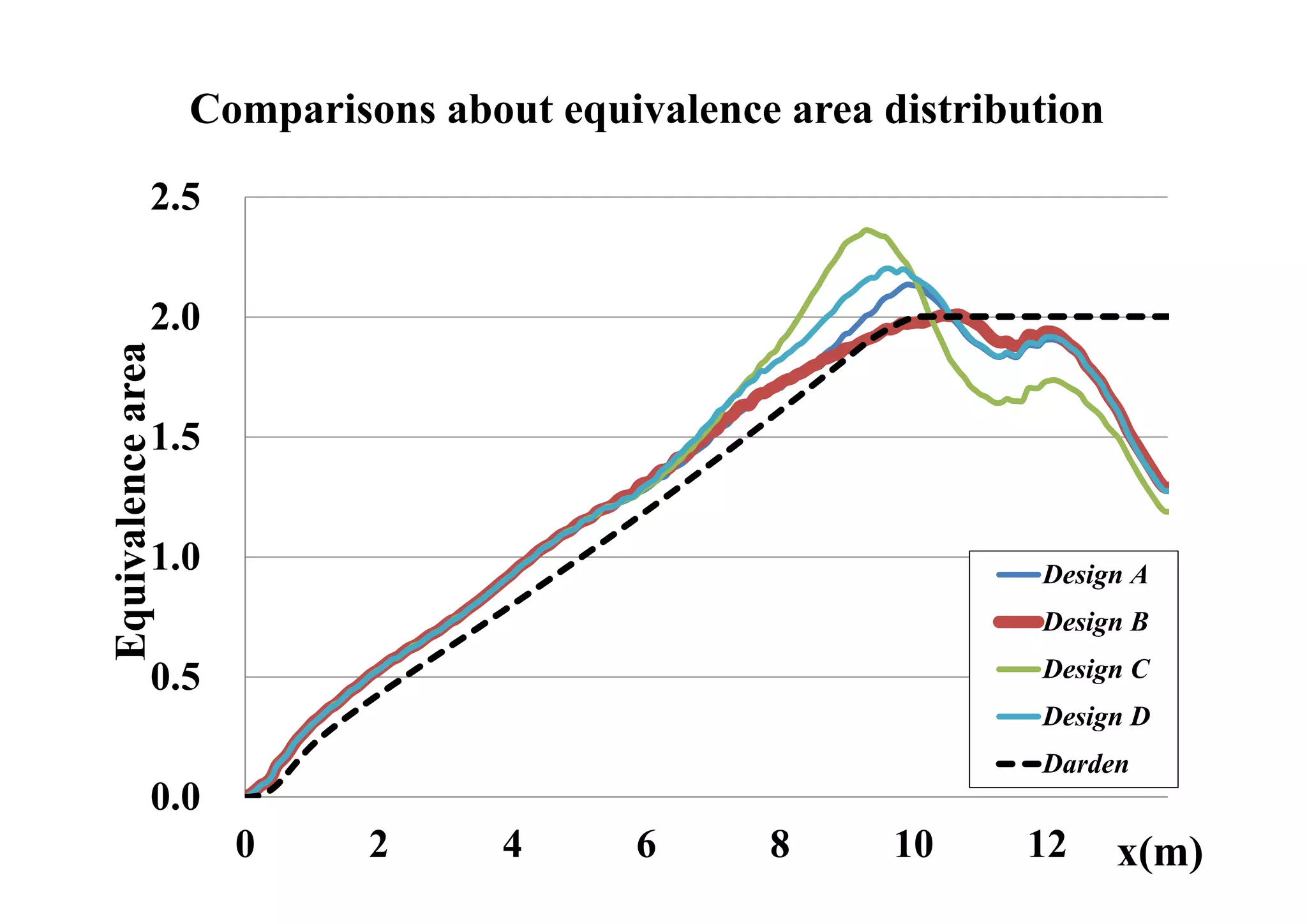
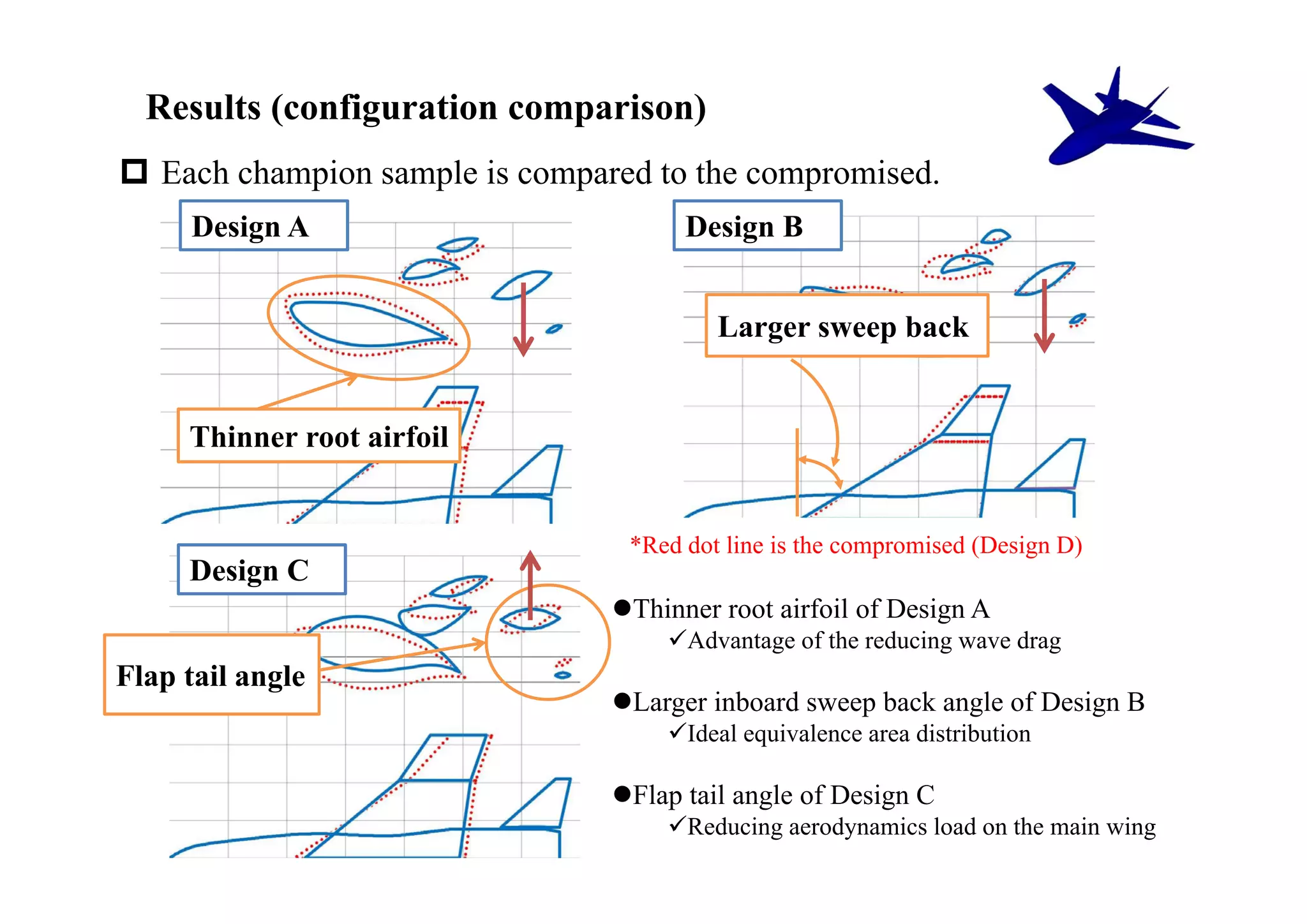
25. Results (waveform on the ground)
 Each champion sample is compared to the compromised.
*Red dot line is the compromised (Design D)
Less different
Design A
among Design A, B, and D
Large different
between Design C and D
L/D ΔP[psf] Wwing[kg]
Design B
Design A 7.02 1.19 612
Design B 6.08 0.97 502
Design C 5.60 1.53 276
Design D 6.77 1.09 691
Design C
Severe trade-off
between ΔP & Wwing

26. Results (Overview about ANOVA)
70% 45%
*a1 *a2 *a3 73%
dv1 inboard sweep dv8 tip t/c
dv2 outboard sweep dv9 aspect ratio
dv3 root twist dv10 root camber(25%c)
Proper range in
dv4 kink twist dv11 root camber(75%c) design space?
dv5 tip twist dv12 kink camber(25%c)
dv6 root t/c dv13 kink camber(75%c)
dv7 kink t/c dv14 tip camber(25%c)

27. Results (Overview about PCP)
Best 5 samples
about L/D
Extracting useful data about each objective
function for the better visualization *p1
Best 5 samples *p2
about ΔP
24 non-dominated solutions data
Best 5 samples
about Wwing *p3

28. Results (design information of better L/D)
*PCP was carried out from best five samples about L/D
 Root camber(dv10, 11) & kink camber(dv12, 13)
 ANOVA
Design A
upper
 Kink twist(dv4) & root t/c(dv6)
 PCP lower
→Small drag around root & sufficient lift around kink
*a1
*p1

29. Results (design information of better ΔP)
*PCP was carried out from best 5 samples about ΔP
 Inboard sweep(dv1) & root camber(dv10) & kink camber(dv14)
 ANOVA
Design B
 Kink twist(dv4) & root t/c(dv6) & kink t/c(dv7)
 PCP upper
lower
→Ideal equivalence area (Ae) distribution
*a2
*p2

30. Comparisons about equivalence area distribution
2.5
2.0
Equivalence area
1.5
1.0 Design A
Design B
0.5 Design C
Design D
Darden
0.0
0 2 4 6 8 10 12 x(m)

31. Results (design information of better Wwing)
*PCP was carried out from best 5 samples about Wwing
 Root t/c(dv6) & AR(dv9) & root camber(dv10) & kink camber(dv12, 13)
 ANOVA
Design C
 Inboard sweep(dv1) & tip twist(dv5) & kink t/c(dv6)upper
 PCP
lower
→Low aerodynamic load on the wing
*a3
*p3

32. Conclusions
 Efficient MDO tool for conceptual design
 MOGA with Kriging model
 MOGA with Kriging model took about 10 days for the total task
 MOGA without Kriging model would take about 160 days in this study
 Trade-off among each objective function
→Severe trade-off between ΔP and wing weight
 ANOVA
ANOVA found the design variables which have effects on each objective functions.
 PCP
PCP showed the global trend of design variables.
 Better L/D → root & kink camber
 Better ΔP → inboard sweep back angle
 Better wing weight → aspect ratio & root t/c
Efficient exploration
Useful design information pool

33. Acknowledgement
• I wish to thank Dr. Yoshikazu Makino, and Dr. Takeshi
Takatoya, researchers in Aviation Program Group/Japan
Aerospace Exploration Agency, for providing their CAE
program and large support. I would like to thank my paper
adviser, Prof. Masahiro Kanazaki, for his guidance, and
support.
• My presentation is supported by the grant from JSASS (Japan
Society of Aeronautics and Space Science).