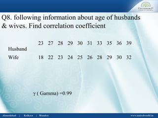
Downloaded 35 times


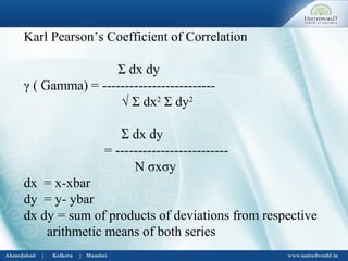
![Karl Pearson’s Coefficient of Correlation
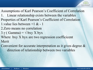
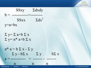
After calculating assumed or working mean Ax & Ay
Σ dx dy – (Σ dx) x( Σ dy)
γ ( Gamma) = --------------------------------
√ [ NΣ dx2
- (Σ dx)2
x [Σ Ndy2
- (Σ dy)2
]
Σ dx dy = total of products of deviation from assumed
means of x and y series
Σ dx = total of deviations of x series
Σ dy = total of deviations of y series
Σ dx2
= total of squared deviations of x series
Σ dy2
= total of squared deviations of y series
N= No. of items ( no. of paired items](https://image.slidesharecdn.com/correlationregression-uwsb-130703063153-phpapp01/85/Correlation-regression-6-320.jpg)
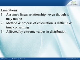
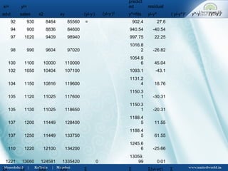
![Karl Pearson’s Coefficient of Correlation
After calculating assumed or working mean Ax &
Ay
Σ dx x Σ dy
Σ dx dy - ----------------
N
γ ( Gamma) = -------------------------
(Σ dx)2
(Σ dy)2
√ [ Σ dx2
- --------- ] x [ Σ dy2
- ------------]
N N](https://image.slidesharecdn.com/correlationregression-uwsb-130703063153-phpapp01/85/Correlation-regression-7-320.jpg)


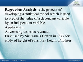
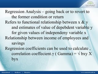
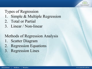
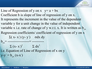

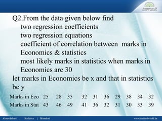

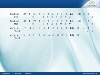

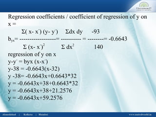
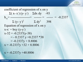

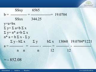


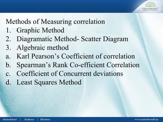
This document discusses correlation and regression analysis. It defines correlation as dealing with the association between two or more variables, and identifies different types including positive/negative, simple/multiple, and linear/non-linear. Regression analysis predicts the value of a dependent variable based on an independent variable. Key aspects covered include Karl Pearson's coefficient of correlation, Spearman's rank correlation coefficient, regression lines, coefficients, and estimating values from the regression equation.


