Downloaded 880 times


This document discusses two-way analysis of variance (ANOVA). It explains that two-way ANOVA allows researchers to study the effects of two independent variables on a single dependent variable. Researchers can test for main effects of each independent variable as well as interactions between the variables. The document provides examples of how to set up a two-way ANOVA study, calculate the relevant statistics, interpret results from ANOVA tables, and draw conclusions about significant main effects and interactions.
Introduction to independent variables as key components in experimental designs.
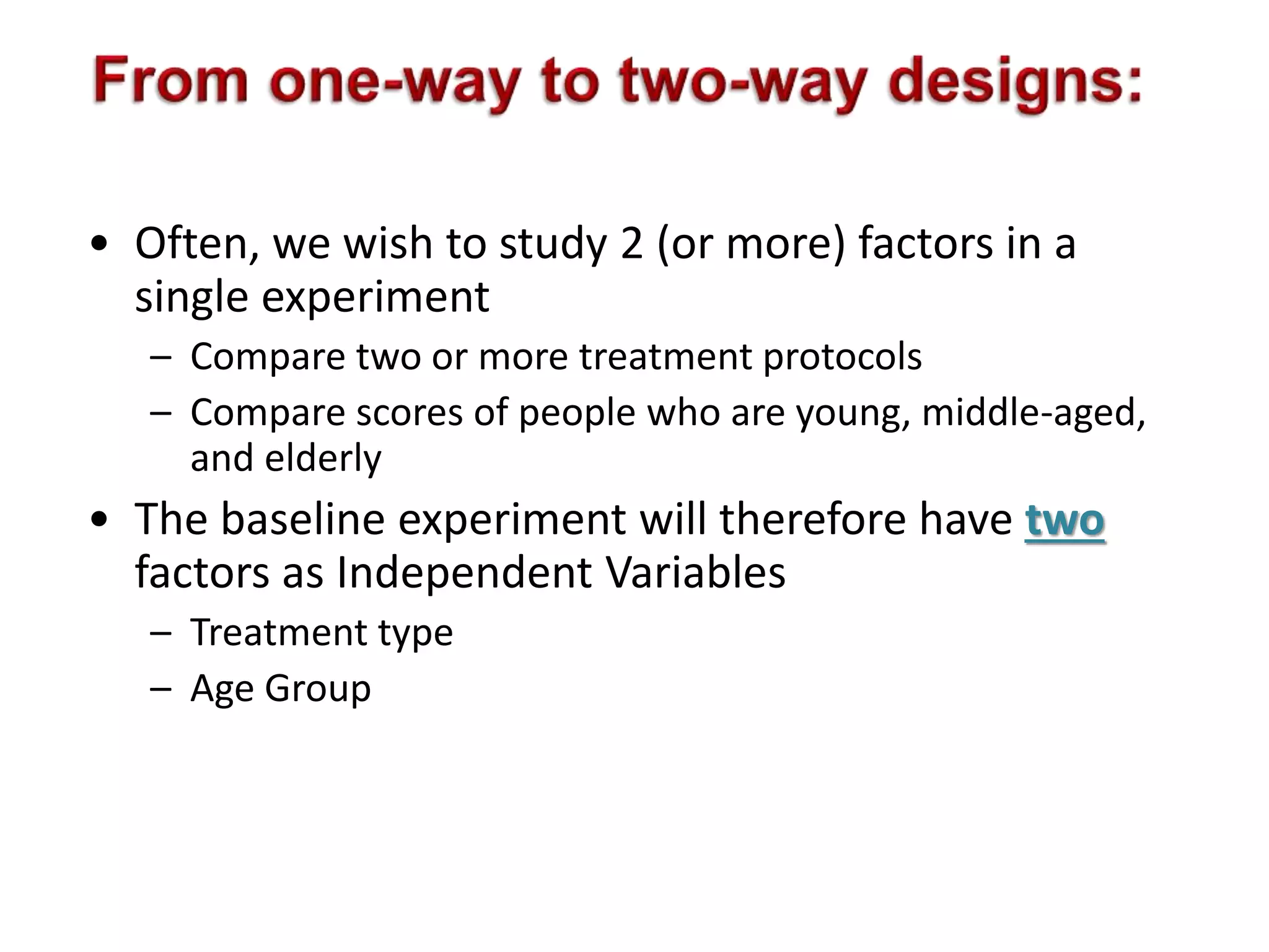
Discusses using two factors in experiments, such as treatment type and age groups.
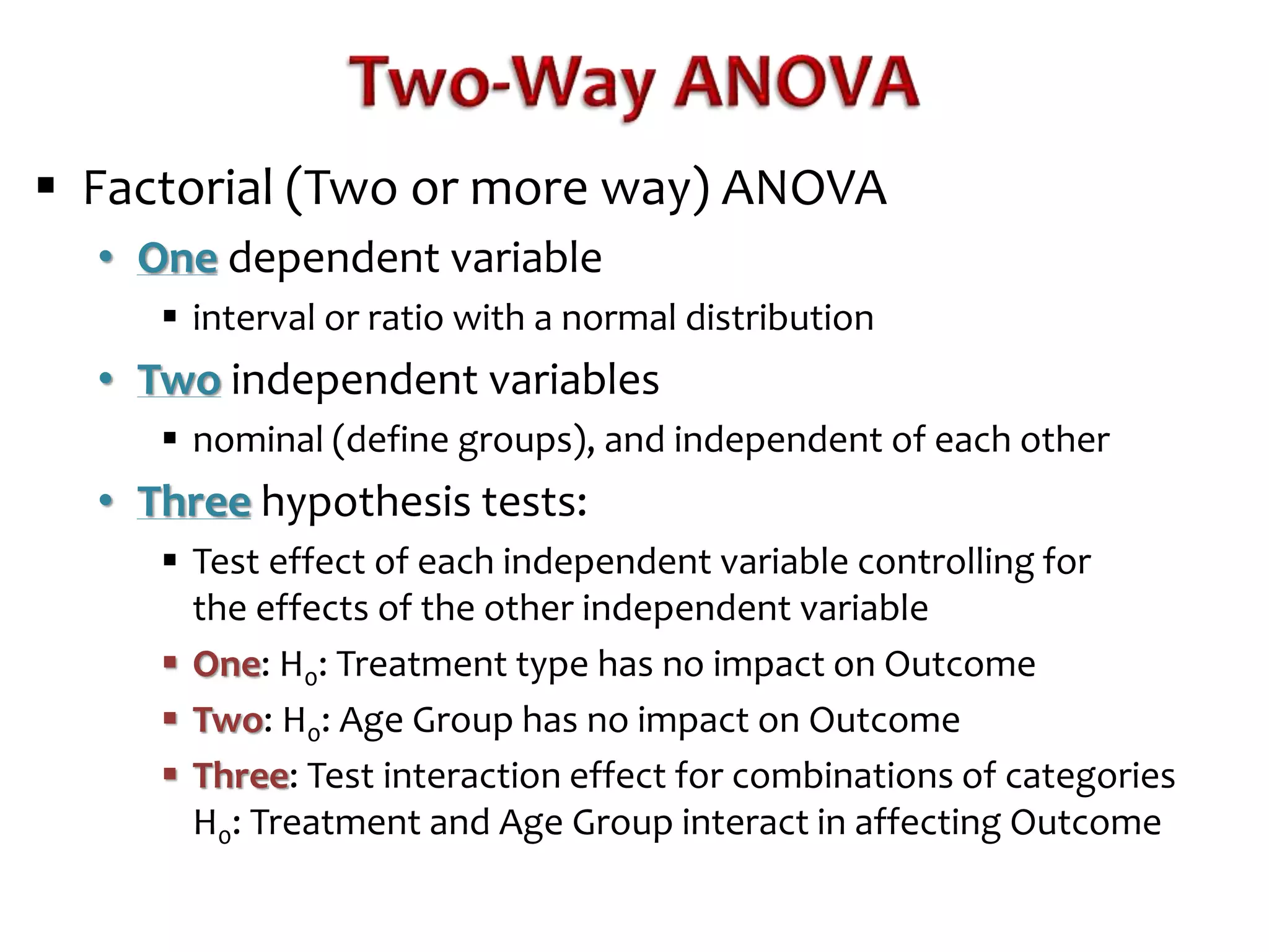
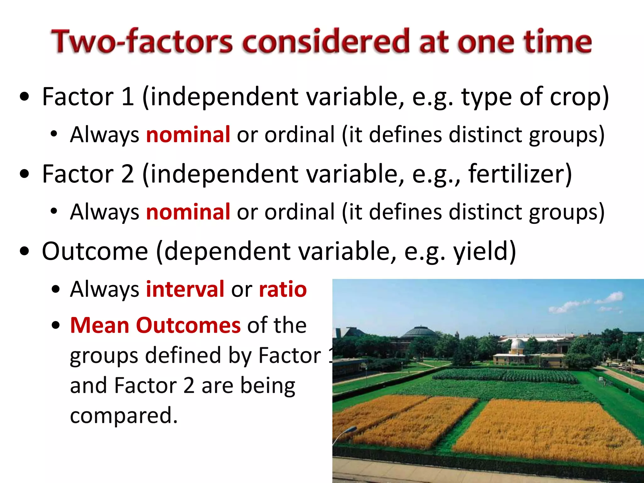
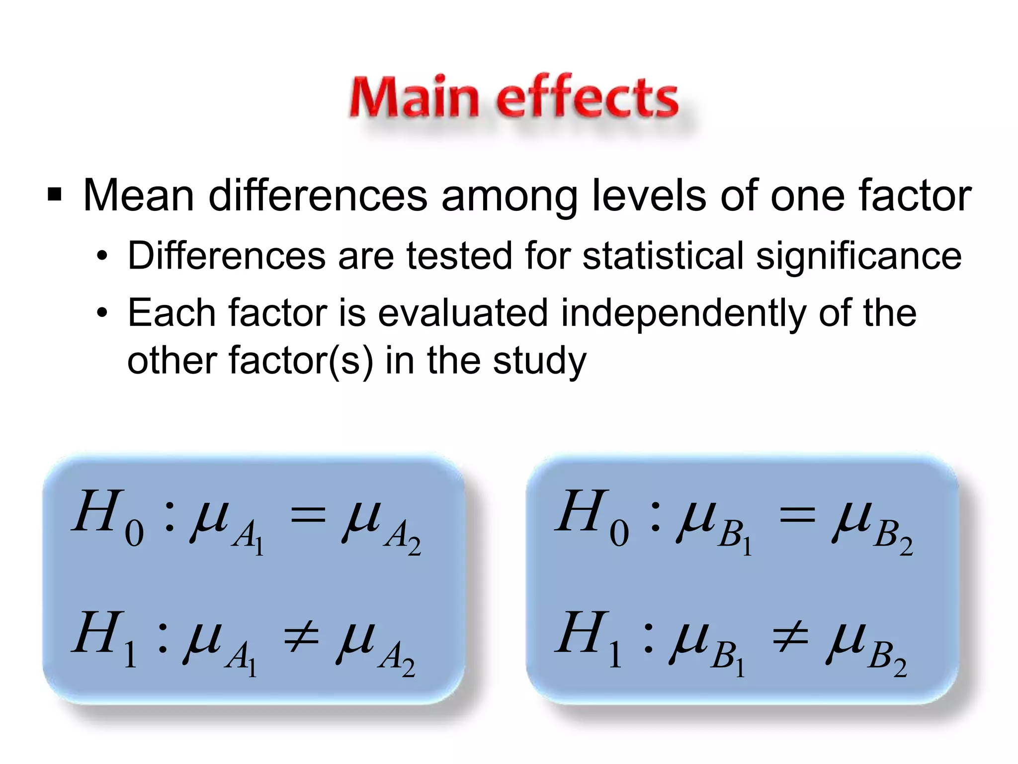
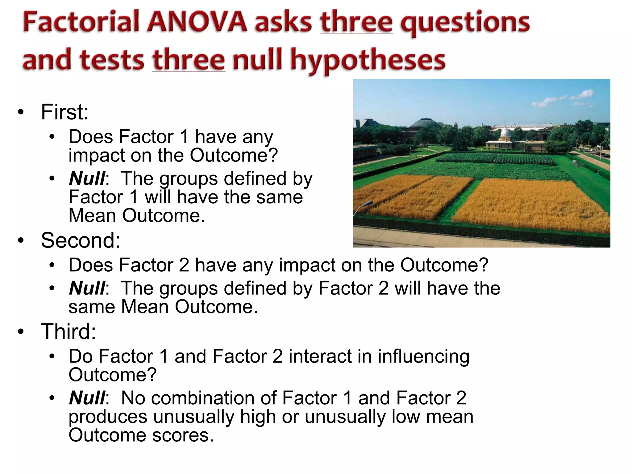
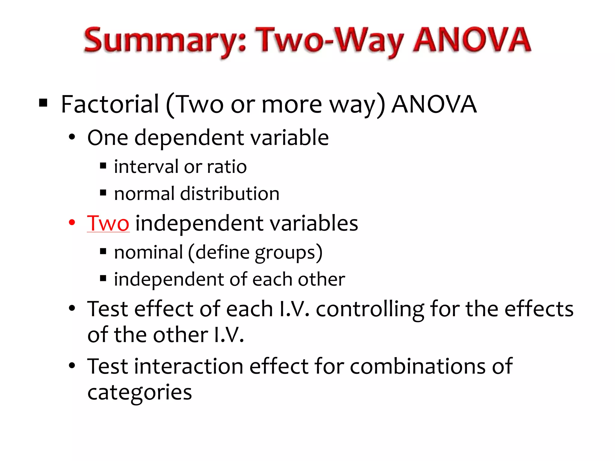
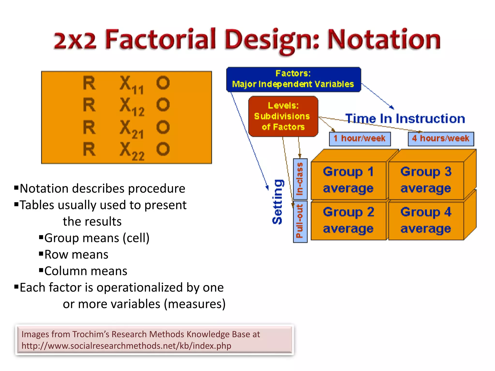
Explains factorial ANOVA with one dependent variable and two independent variables, including hypotheses.
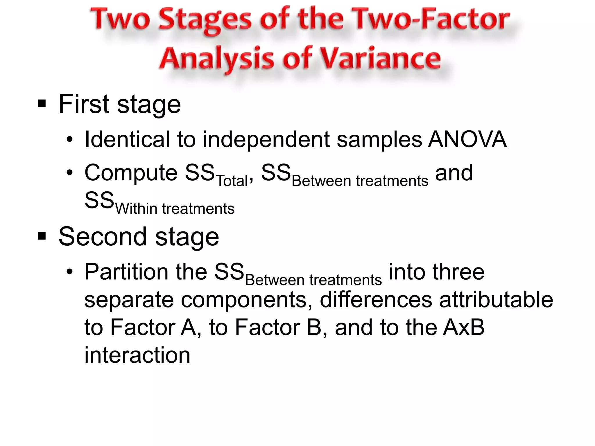
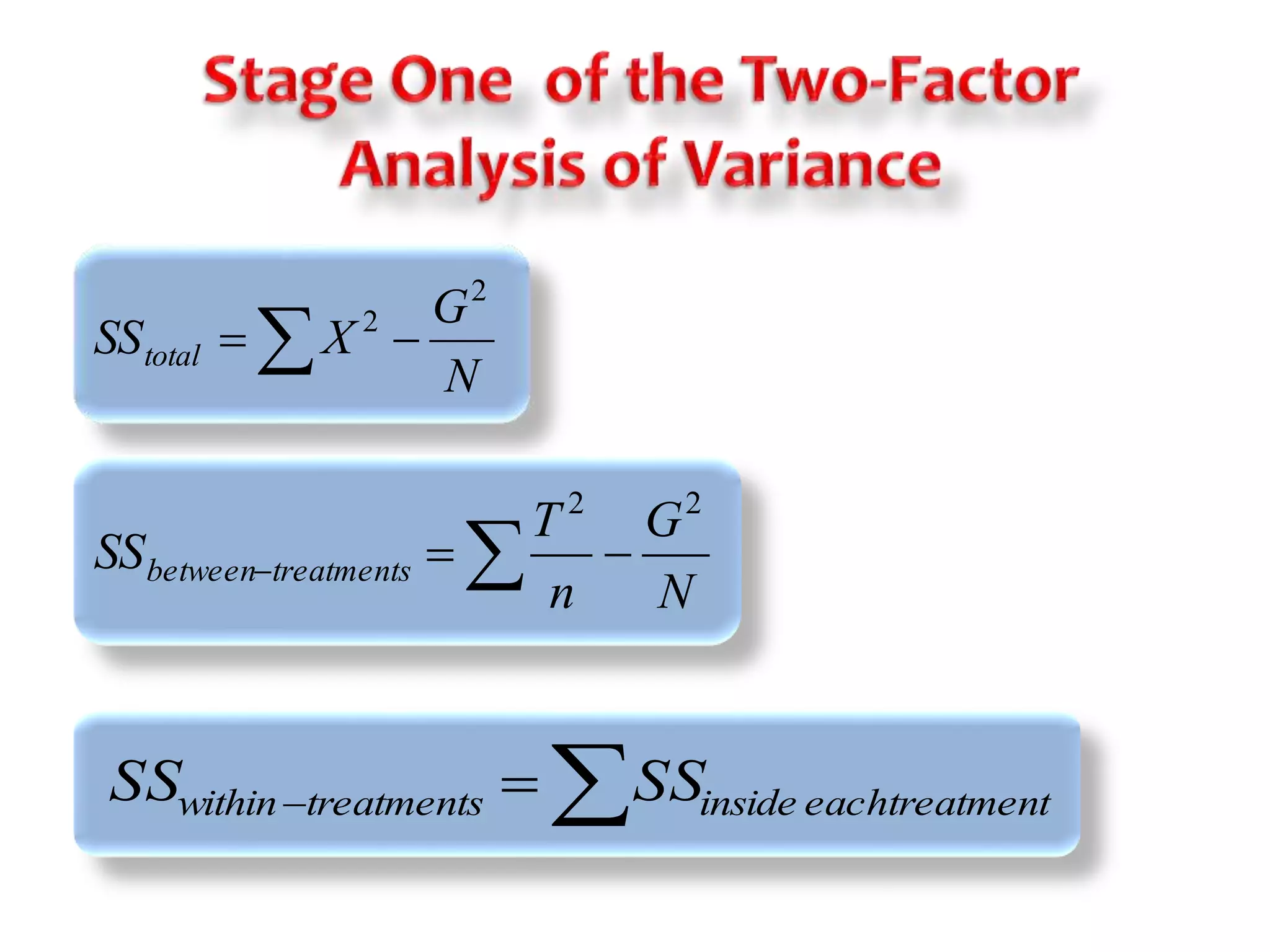
Details the stages in calculating ANOVA, including total and treatment variability.
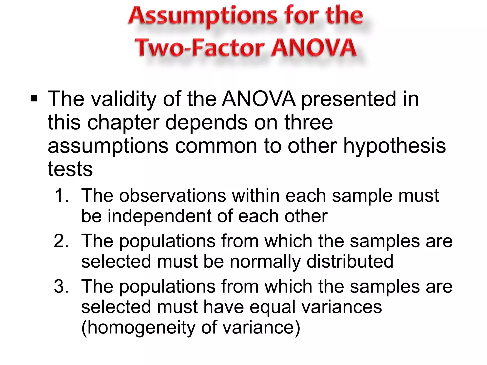
Outlines necessary assumptions for ANOVA: independence, normal distribution, and equal variances.
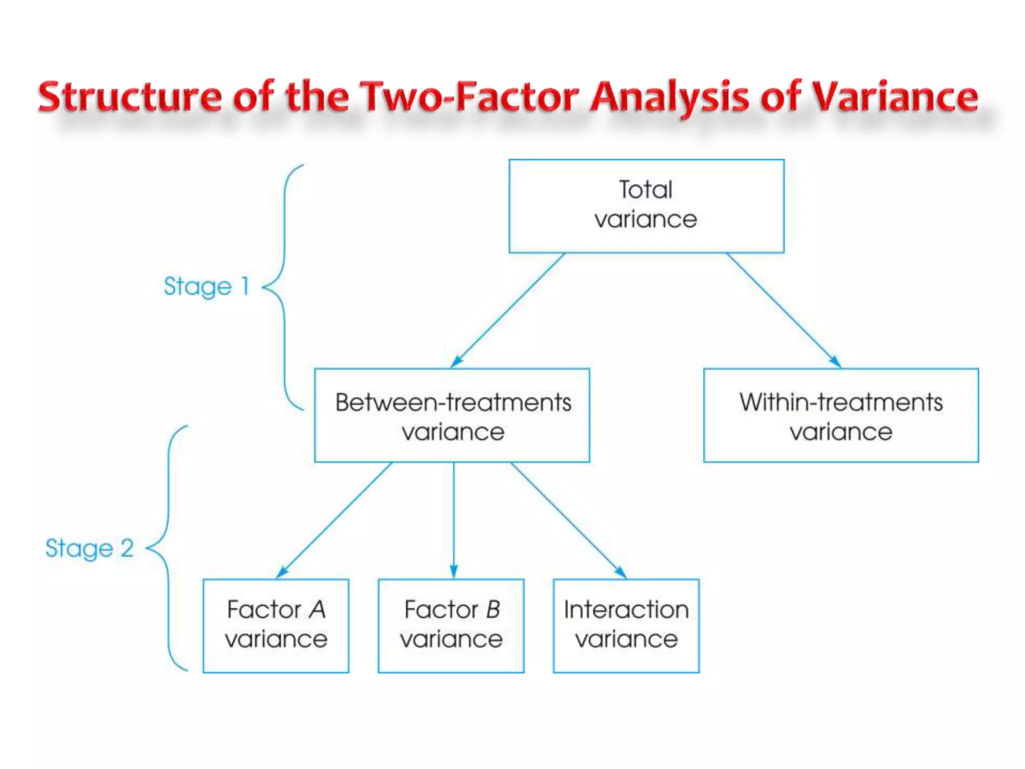
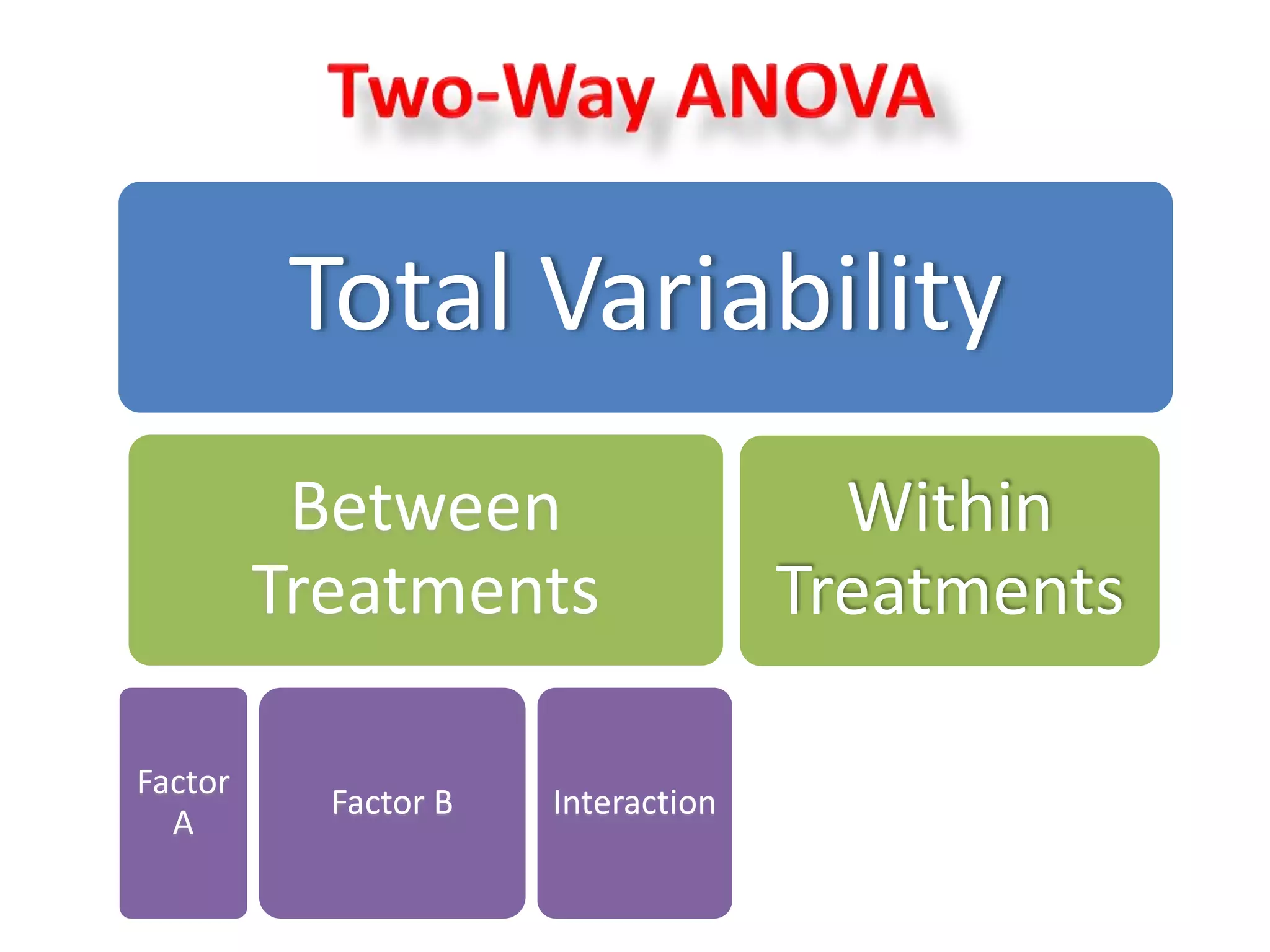
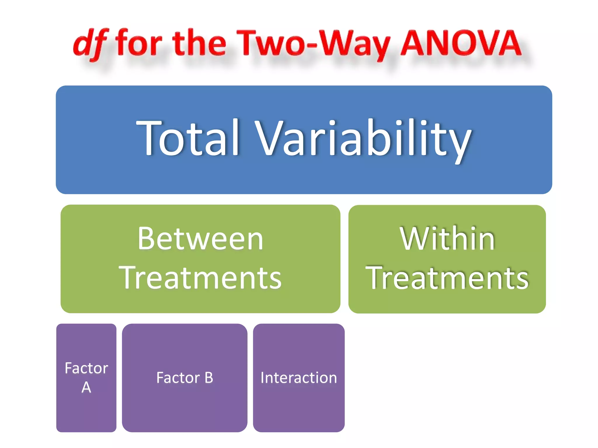
Visual representation of total variability in treatments comprising within and between treatments.
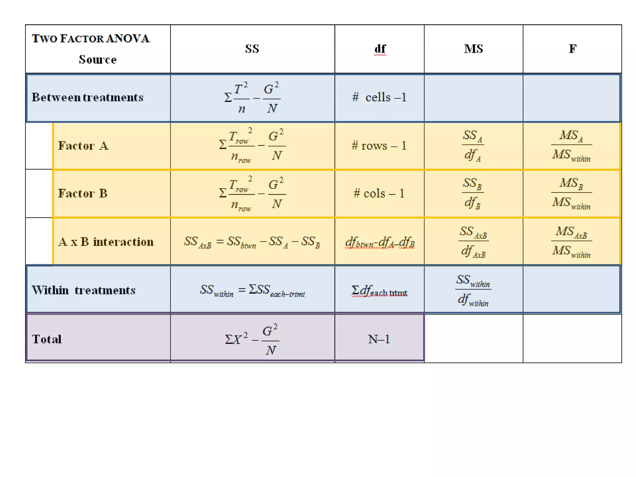
Details calculations for total, between, and within treatments regarding sum of squares.
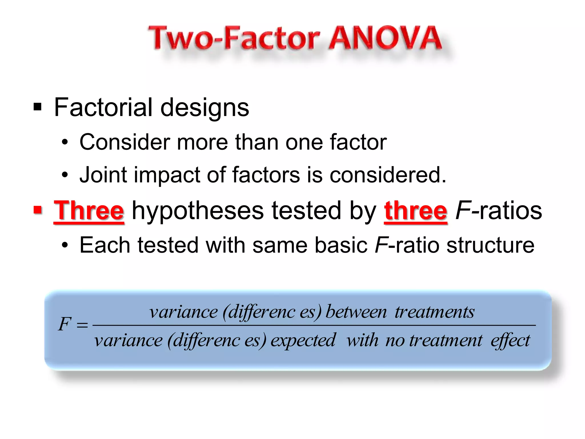
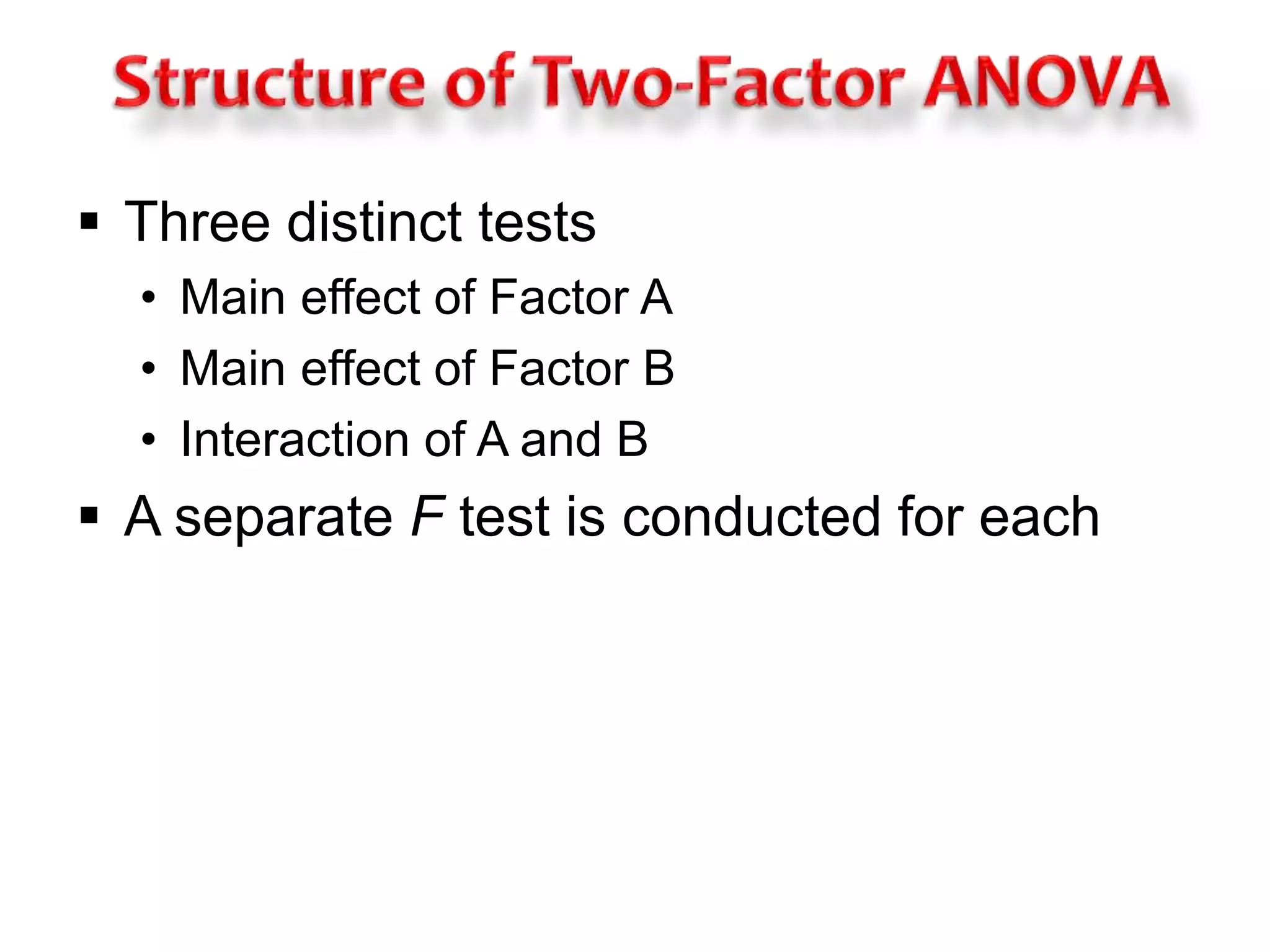
Describes factorial designs with multiple factors and the hypothesis testing structure.
Introduces independent and dependent variables within factorial designs and their significance testing.
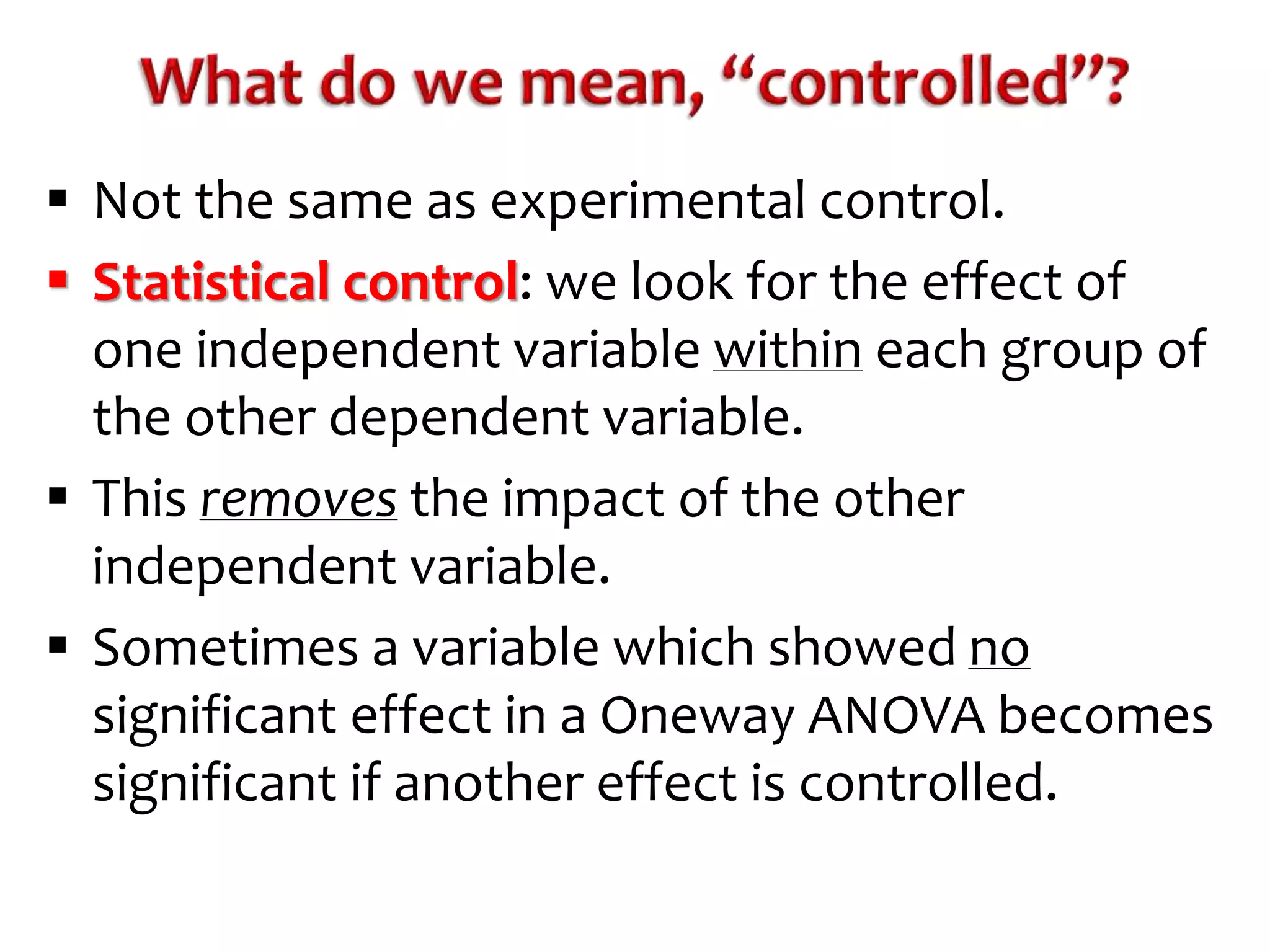
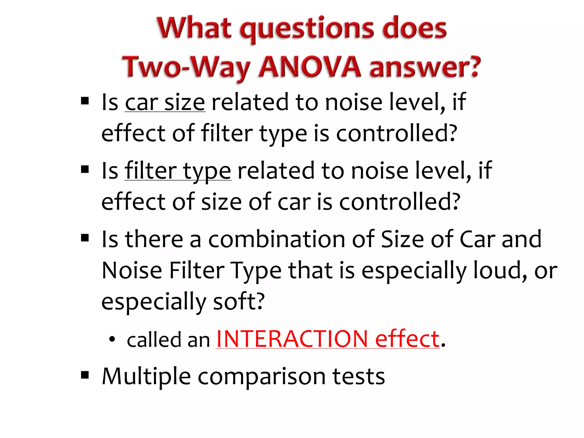
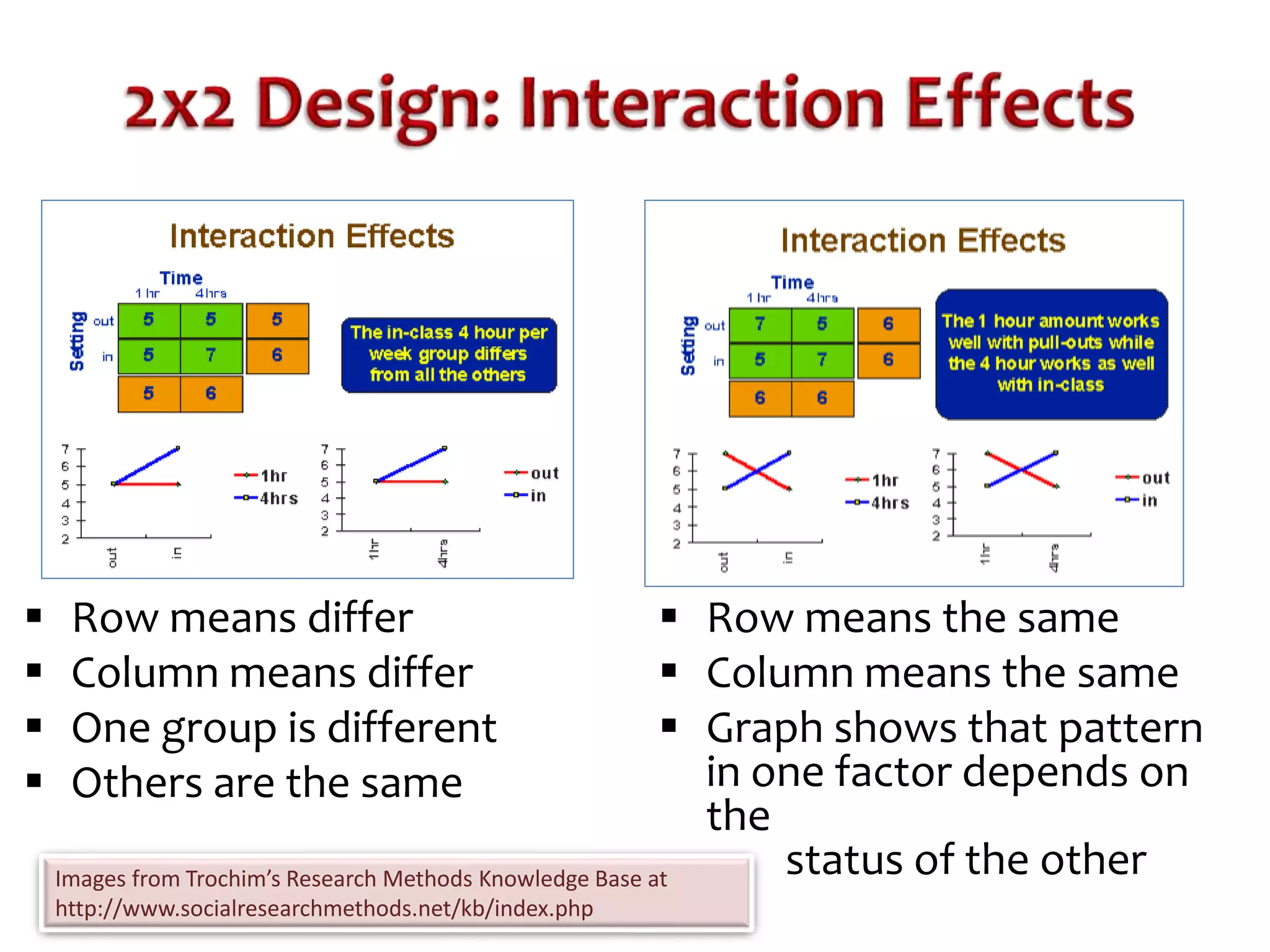
Explains statistical control in two-way ANOVA and the significance of interaction effects.
Discusses the impact of each independent variable and their potential interactions on outcomes.
Illustrates the evolution from one-way to two-way ANOVA with practical examples.
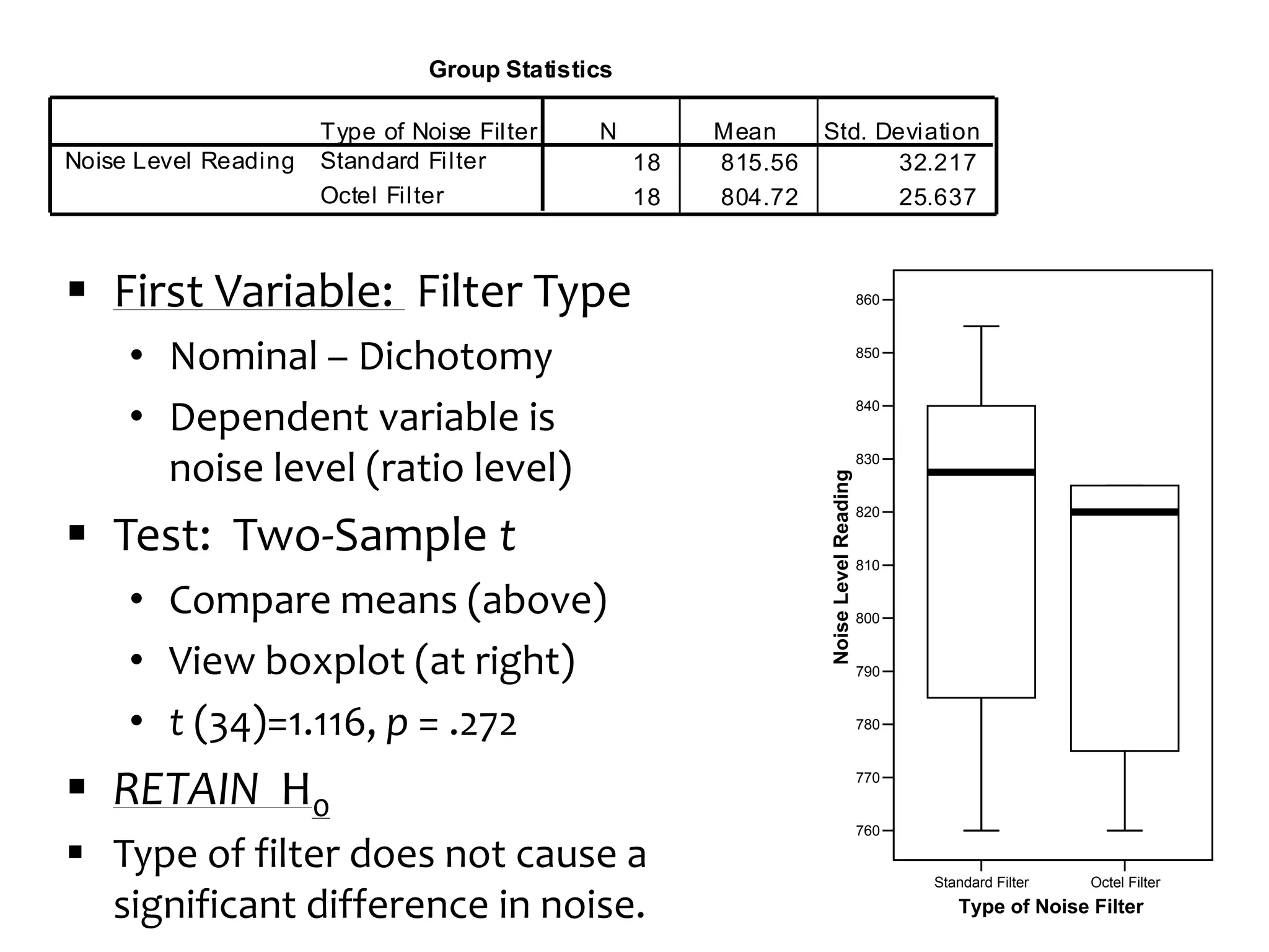
Analyzes noise level readings based on filter types using independent sample t-test for significance.
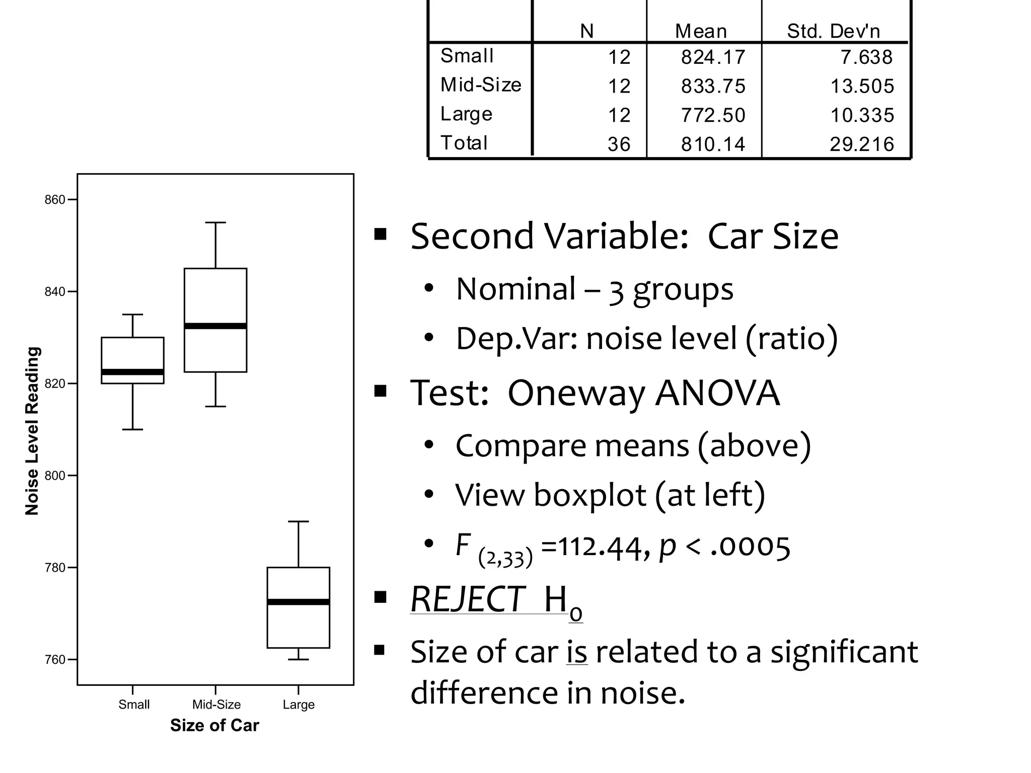
Examines the significance of car size on noise levels using Oneway ANOVA and results.
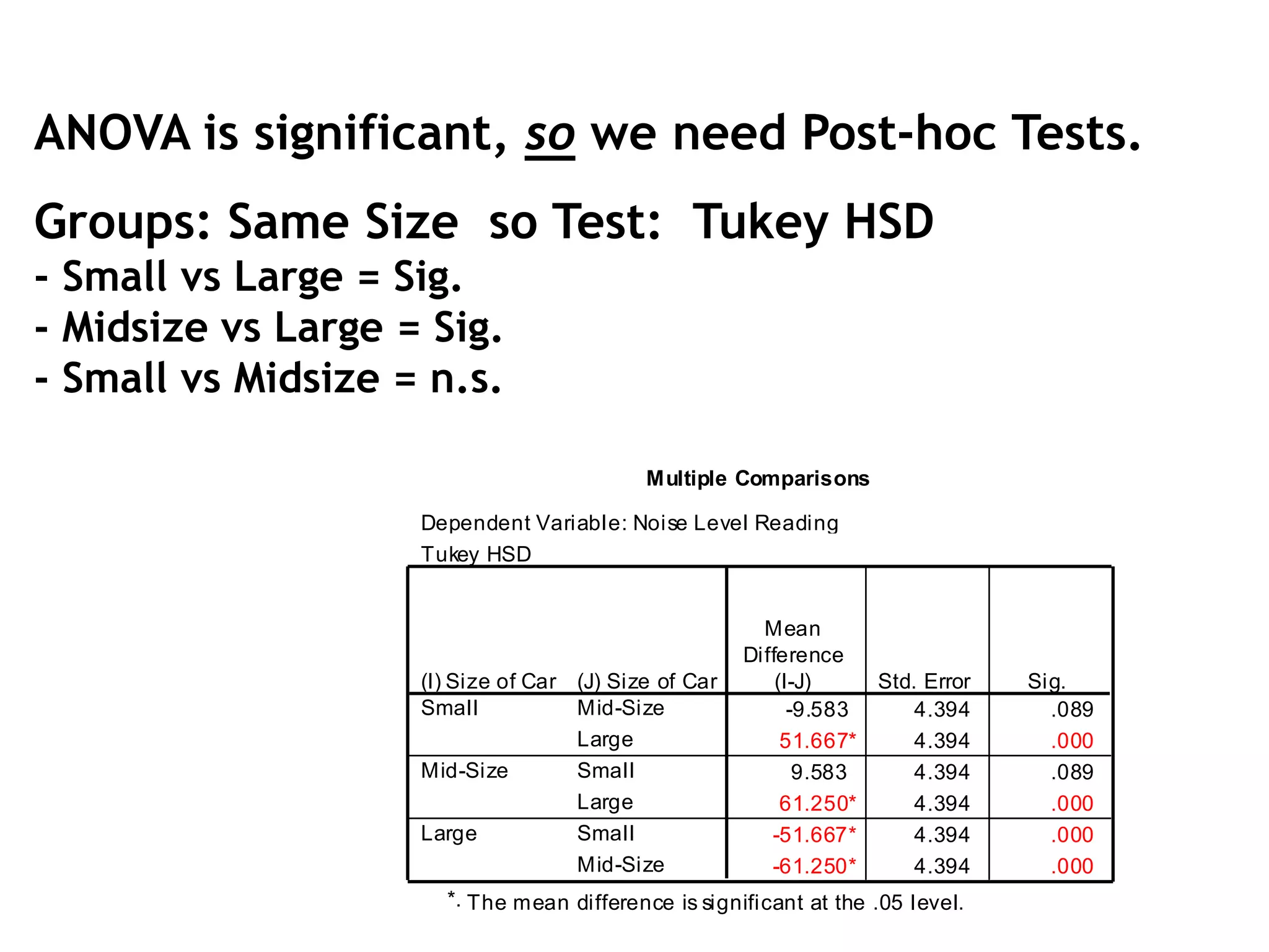
Describes the significance of ANOVA results necessitating further post-hoc tests for comparisons.
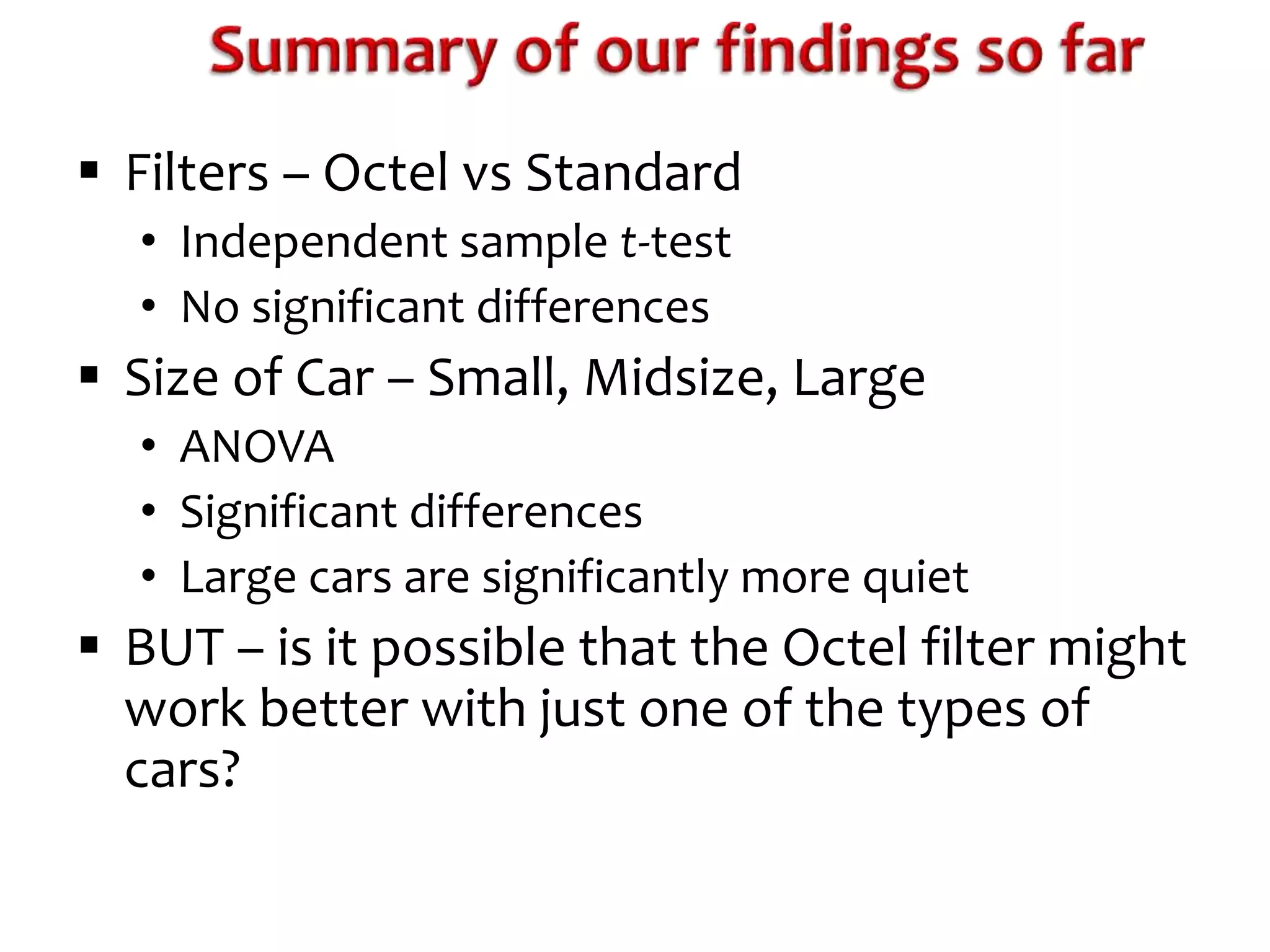
Summarizes findings on noise level effects related to filter types and car sizes.
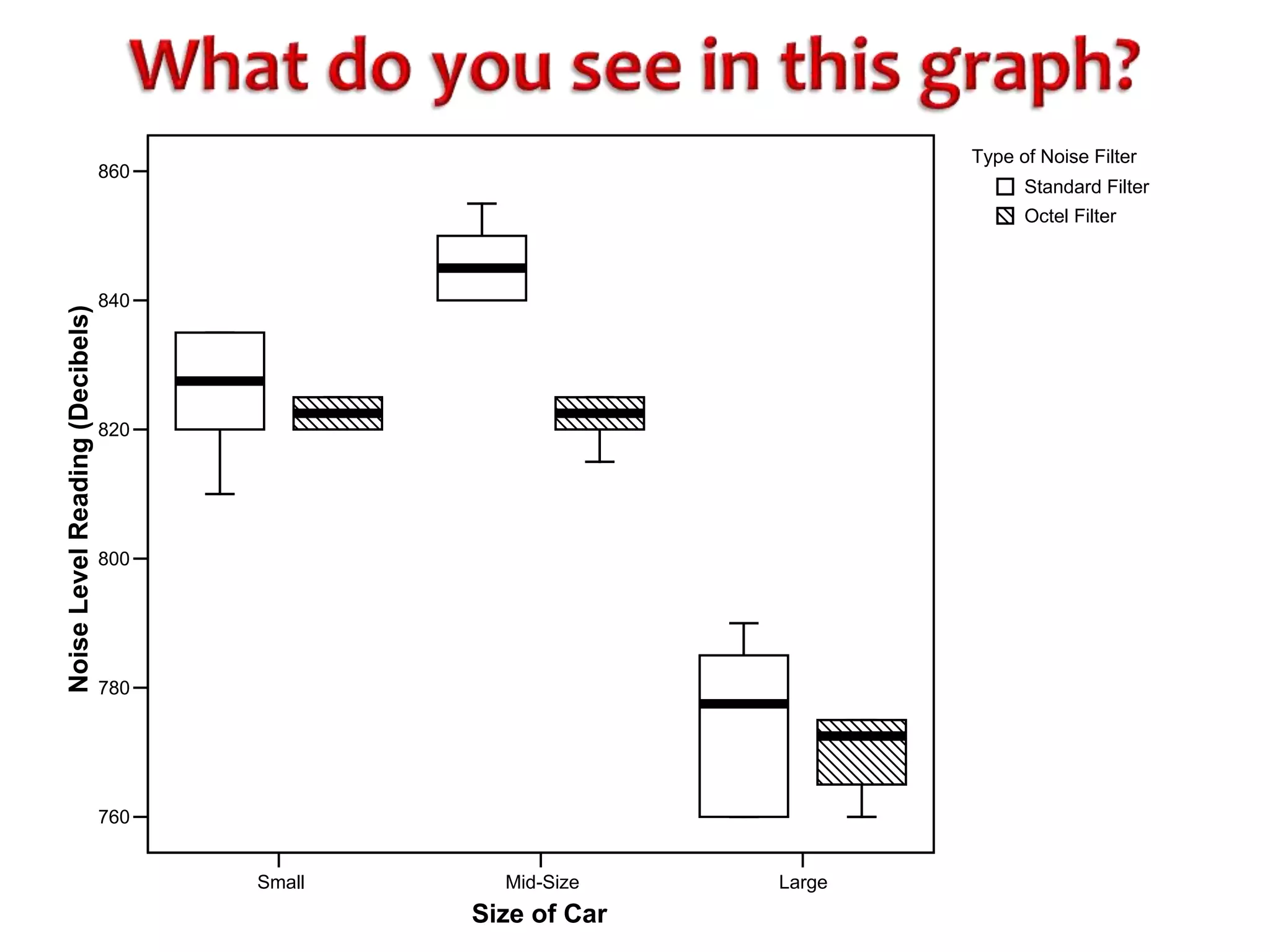
Investigates the interaction effects between filter types and car sizes on noise levels.
Illustrates noise level readings across different car sizes and filter types.
Revisits the structure and testing mechanisms of a factorial ANOVA for outcomes.
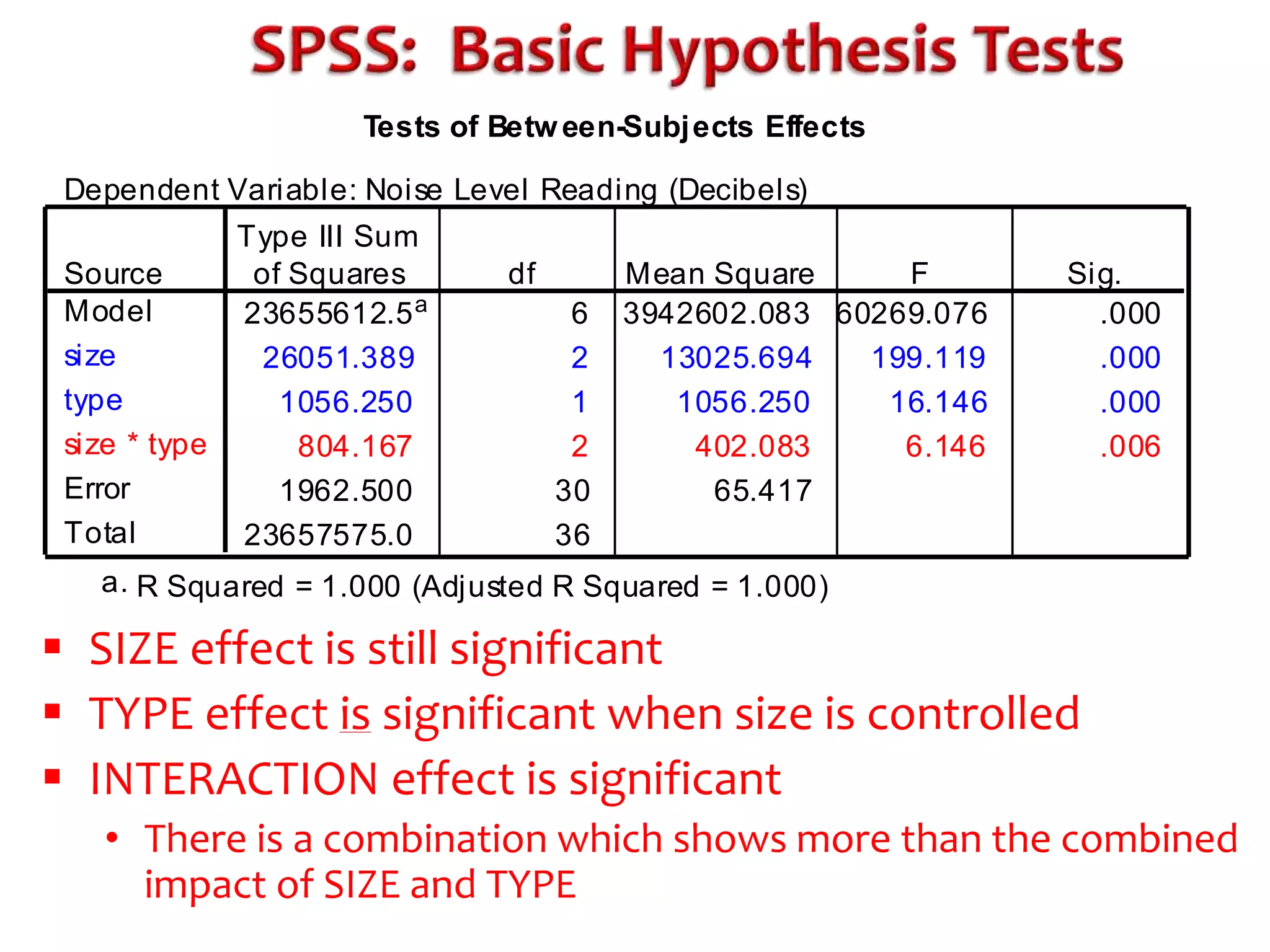
Outlines tests for between-subject effects in factorial ANOVA, including significance levels.
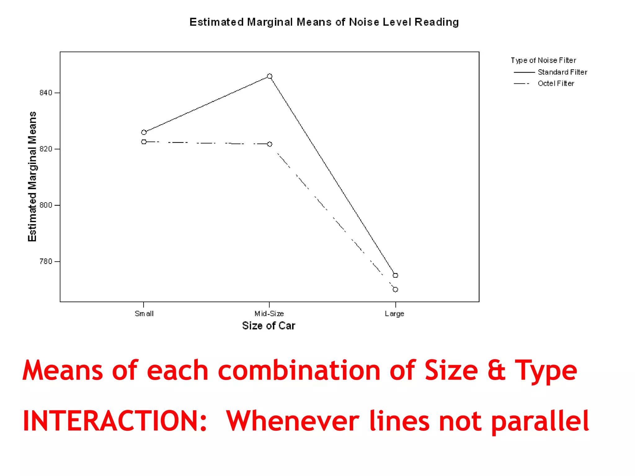
Analyzes means of combinations in factors for interaction effects in ANOVA.
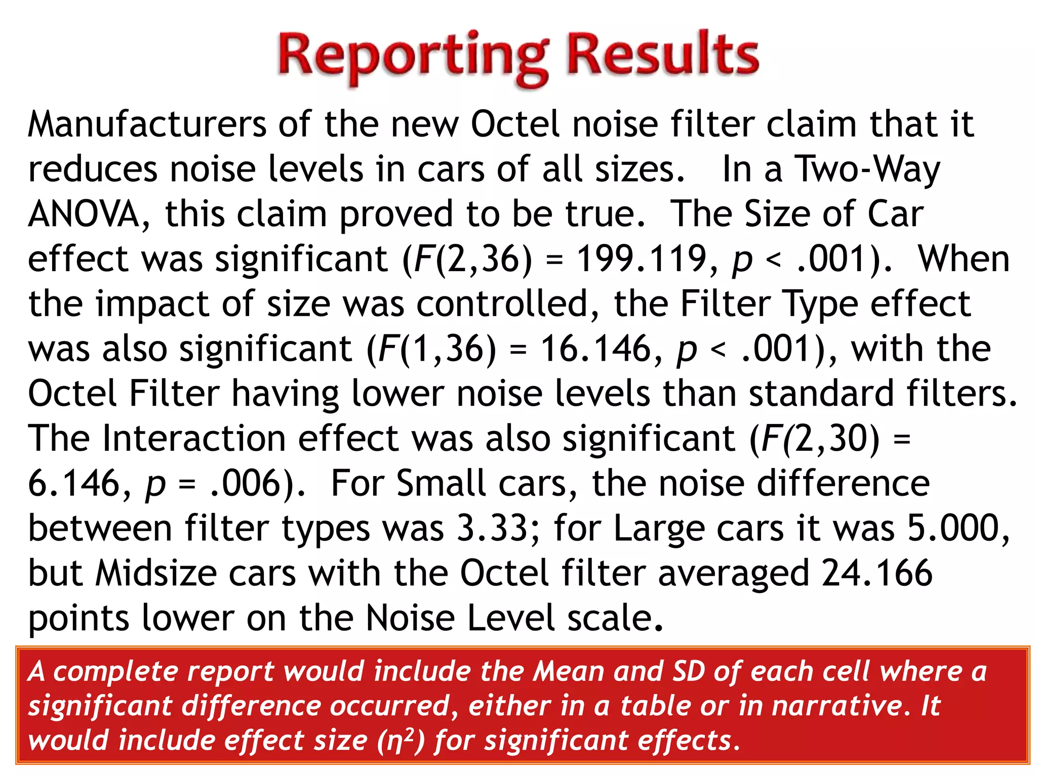
Discusses proper reporting of ANOVA results, including significance and effect sizes.
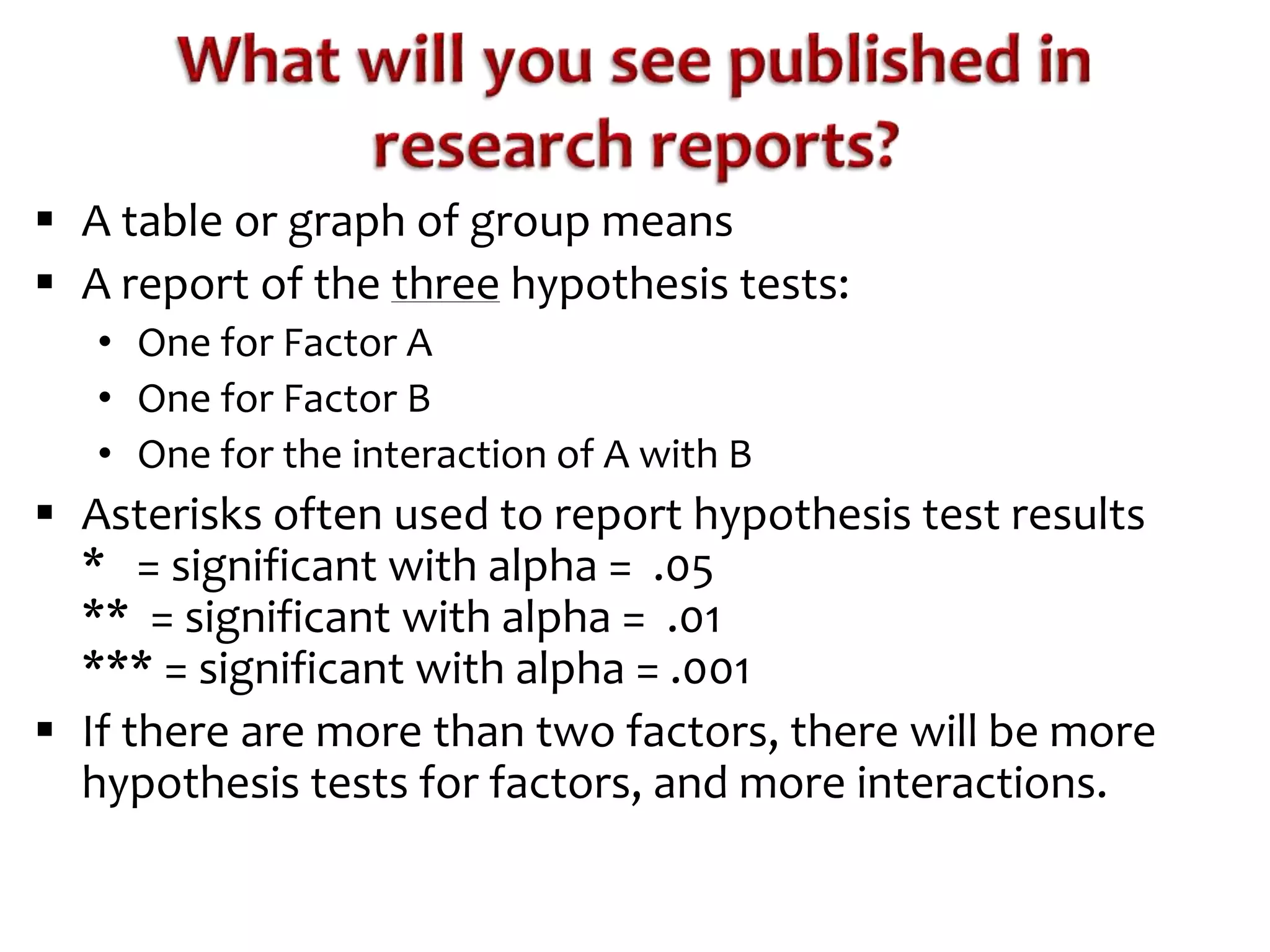
Summarizes necessary reports and tests indicating statistical outcomes and their significance.
Visual representation of total variability between treatments and interactions in designs.
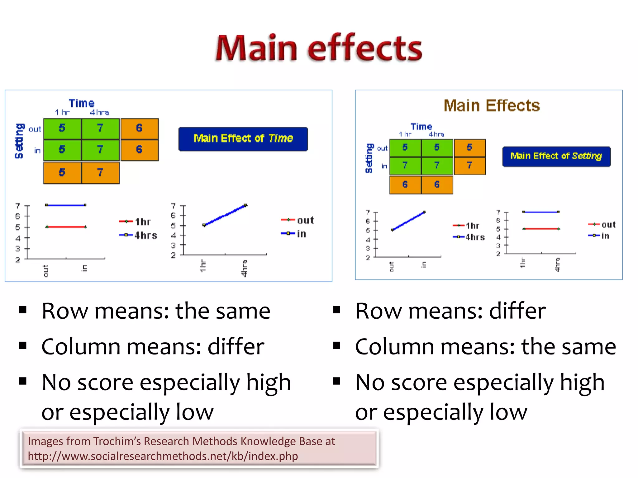
Details on conducting tests for main effects of each independent variable in ANOVA.
Notes on how to present and describe statistical findings in tabular form.
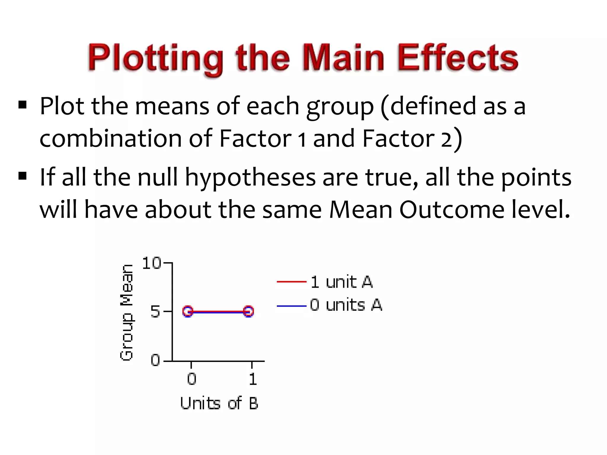
Explains the importance of plotting means to visualize group differences in outcomes.
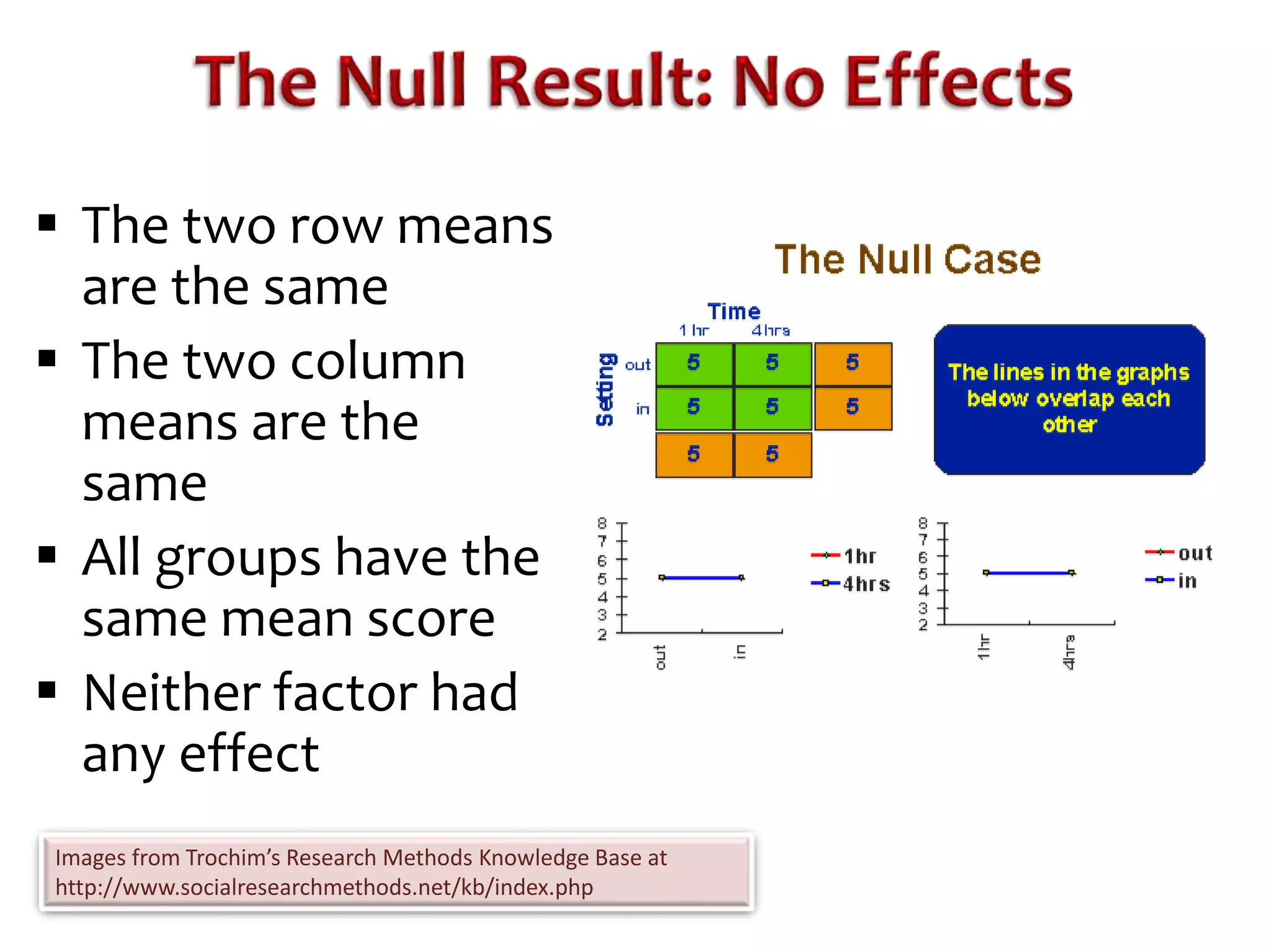
Demonstrates expected results in the absence of effect across group means.
Discusses scenarios where outcomes display no significant effects based on means.
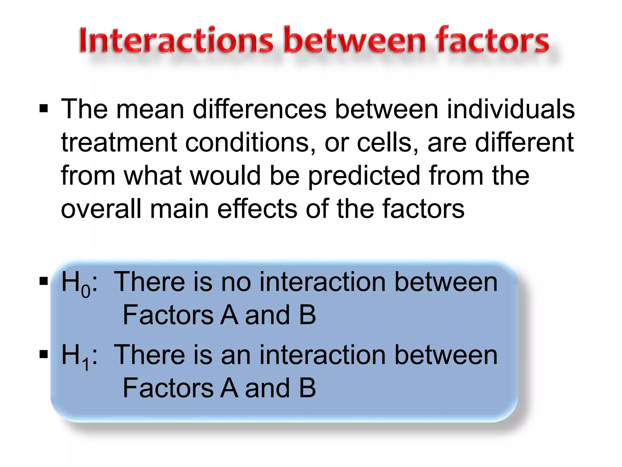
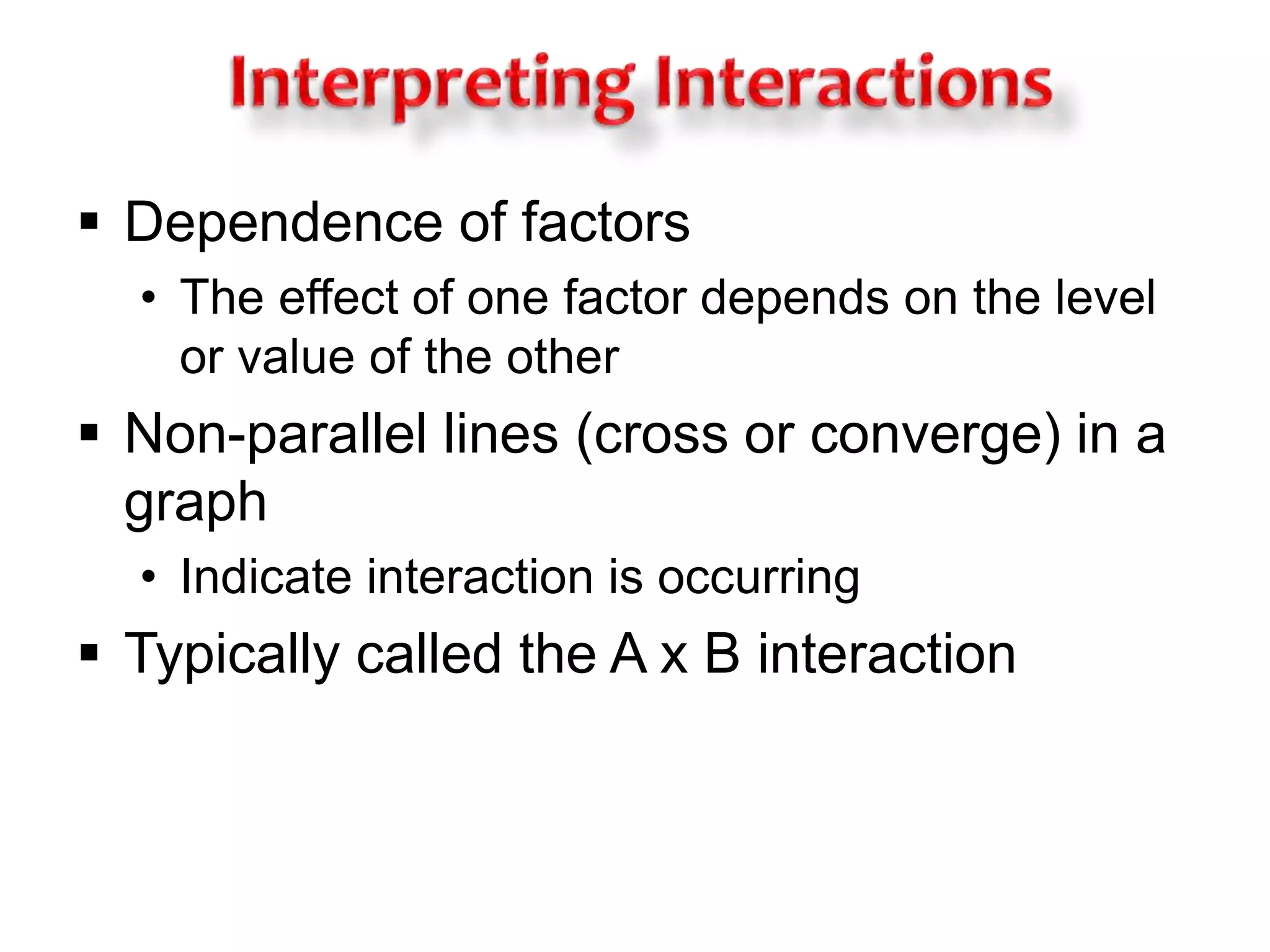
Explains the hypotheses related to interaction effects among factors in ANOVA.
Reviews identification of relationships dependent on various factor levels in analysis.
Emphasizes the use of non-parallel lines in graphs as indicators of interaction effects.
Revisits total variability concepts involving treatments and their interactions.
Encourages practical problem-solving to understand ANOVA computations.
Repeats equations relevant to sum of squares computations in ANOVA.
Revisits the concept of total variability within treatments and their distribution.
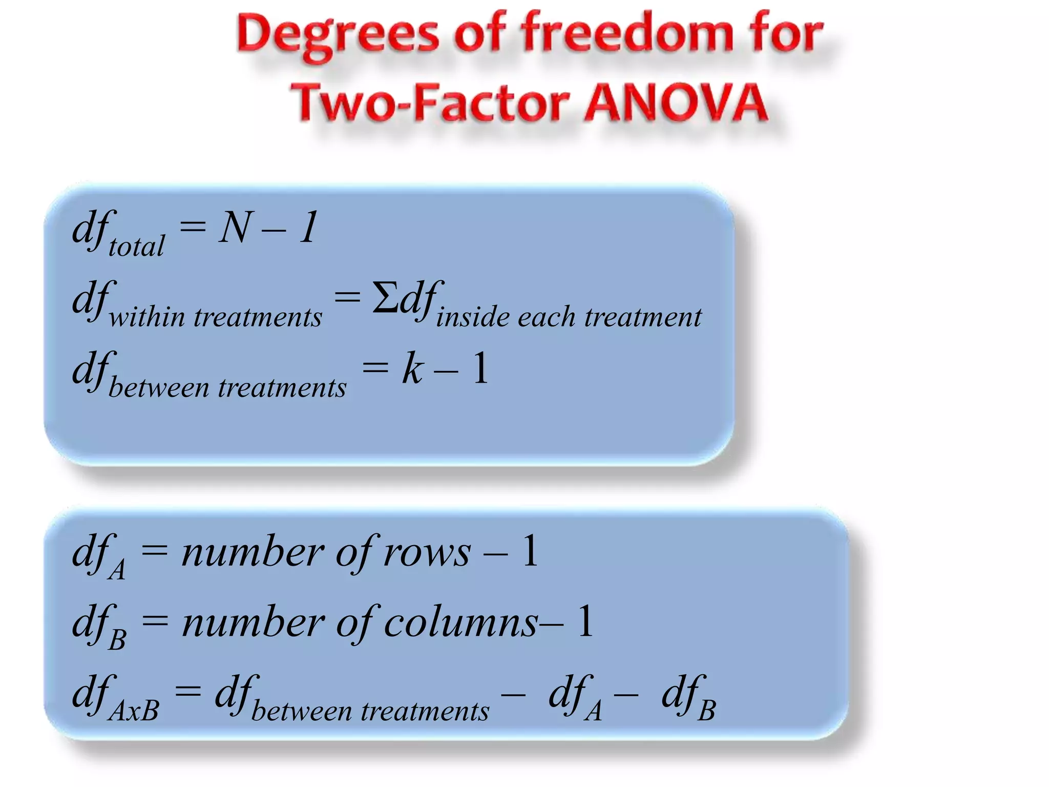
Details formulas related to degrees of freedom within the context of ANOVA calculations.
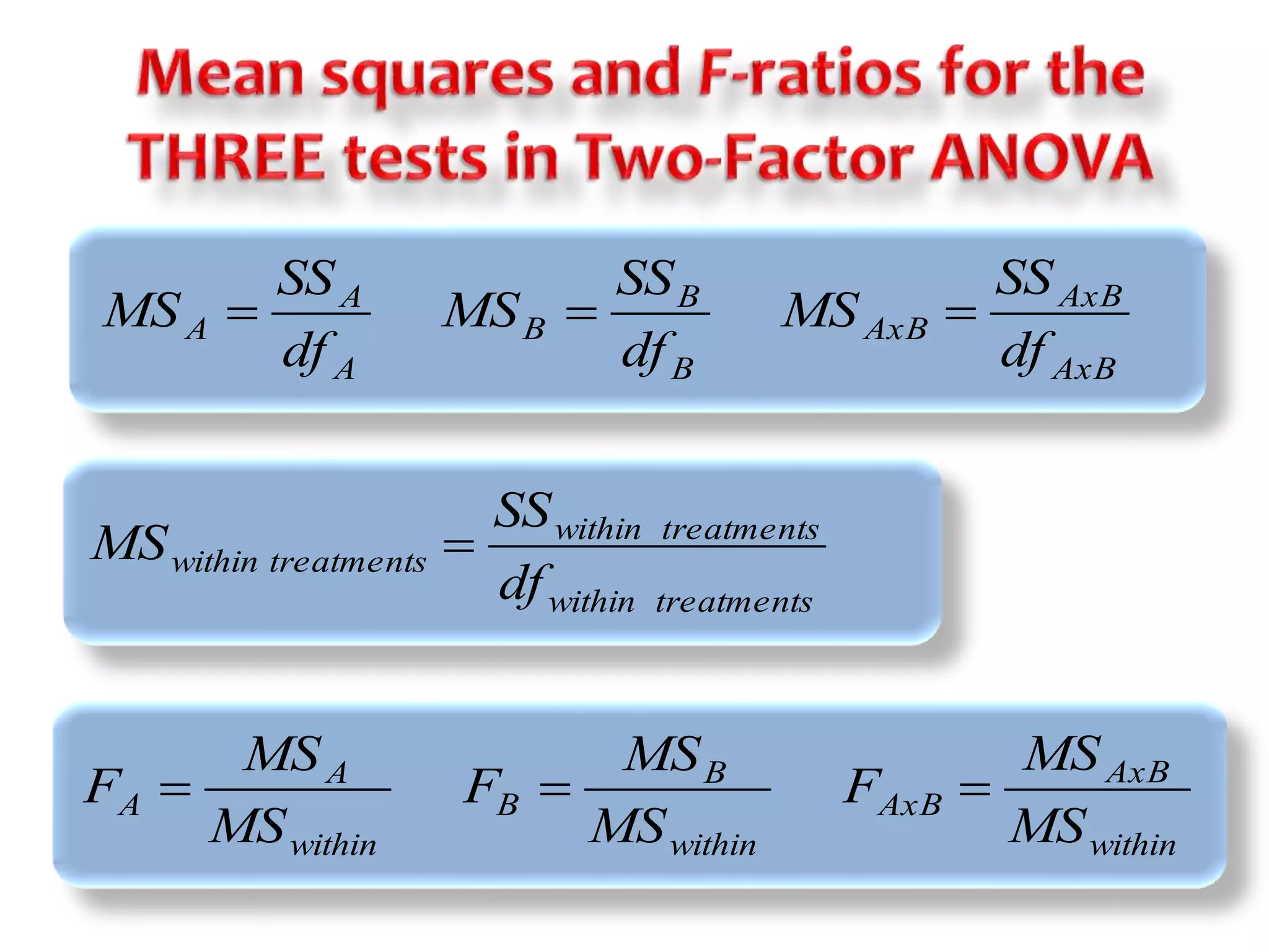
Explains the calculations for mean squares and F-ratios for statistical analysis.
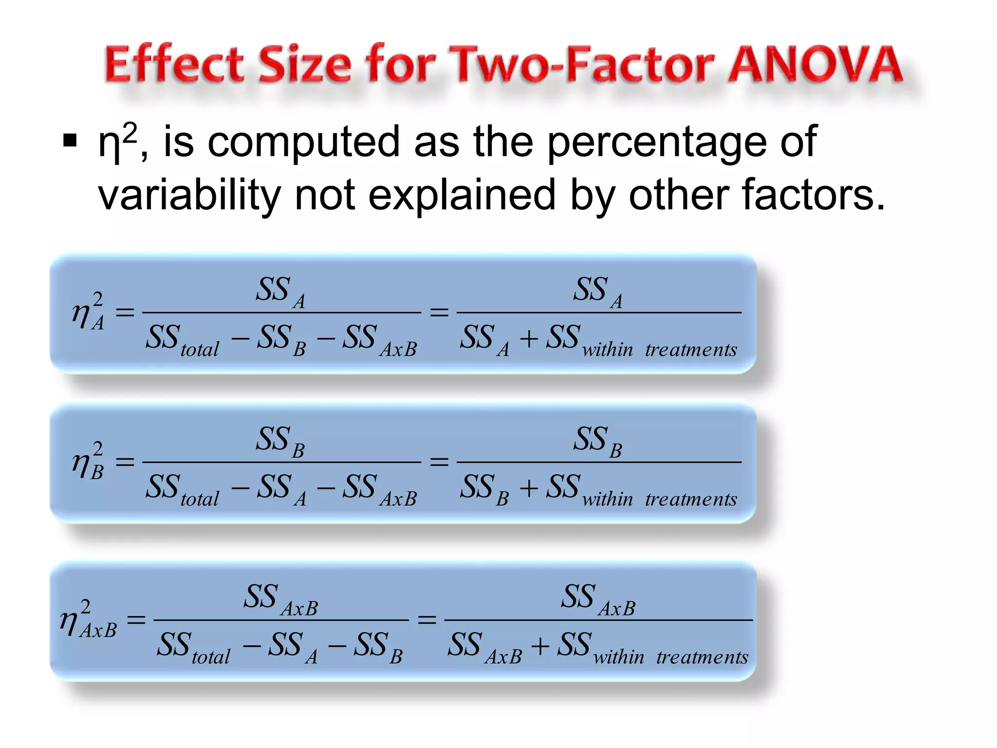
Describes how to calculate effect sizes for various elements in factorial designs.
Wraps up the importance of understanding independent variables in experimental designs.