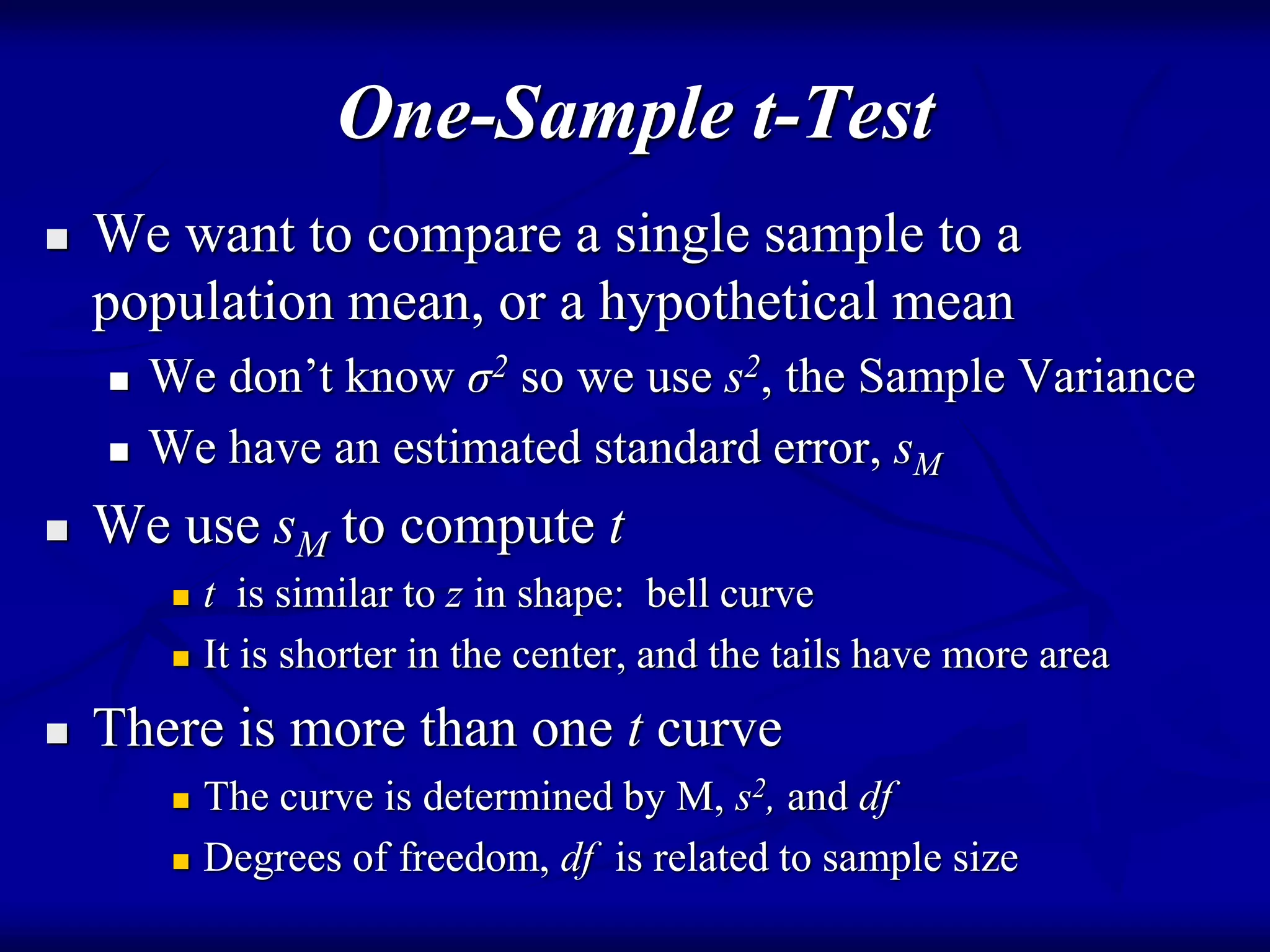
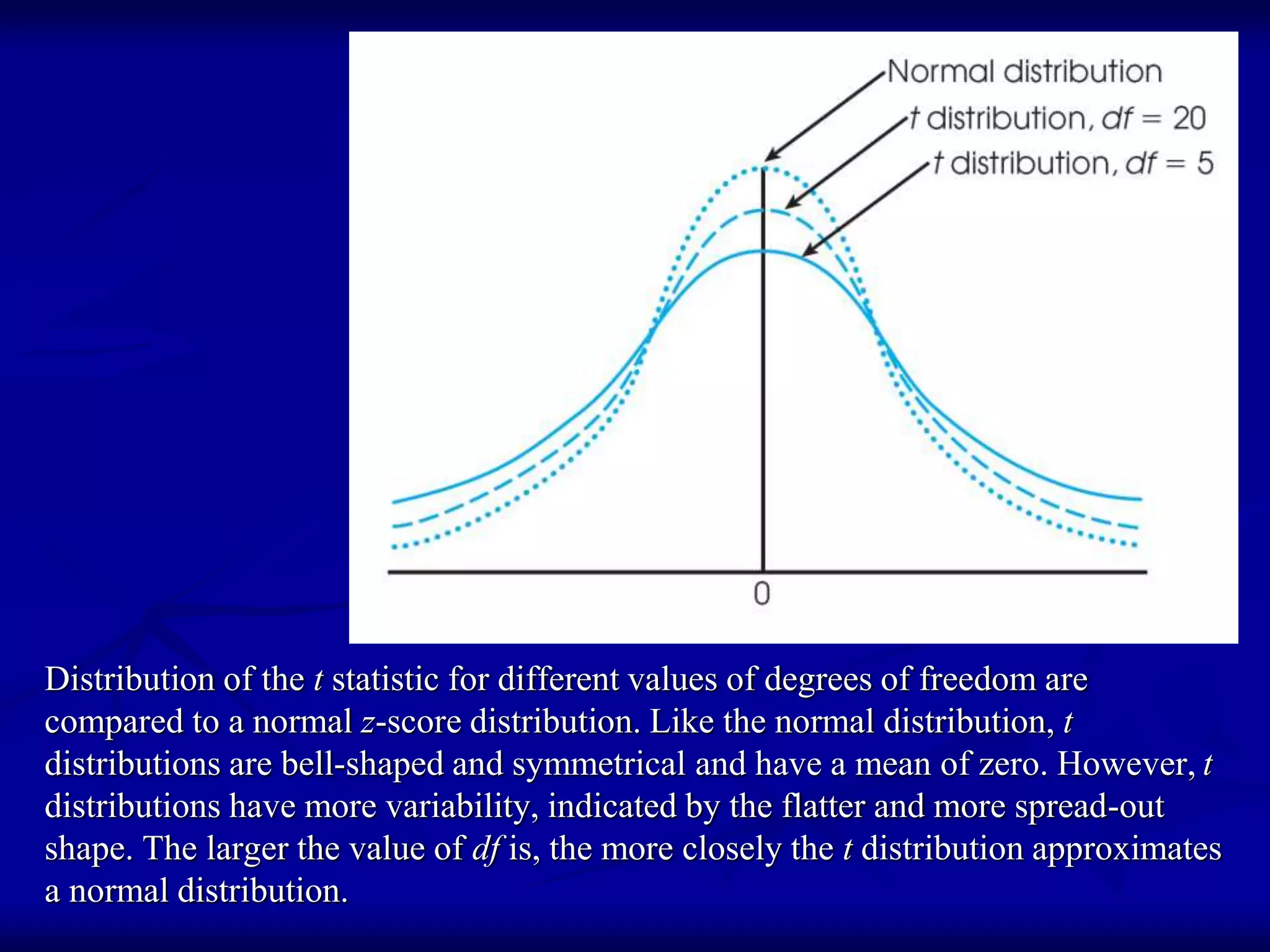
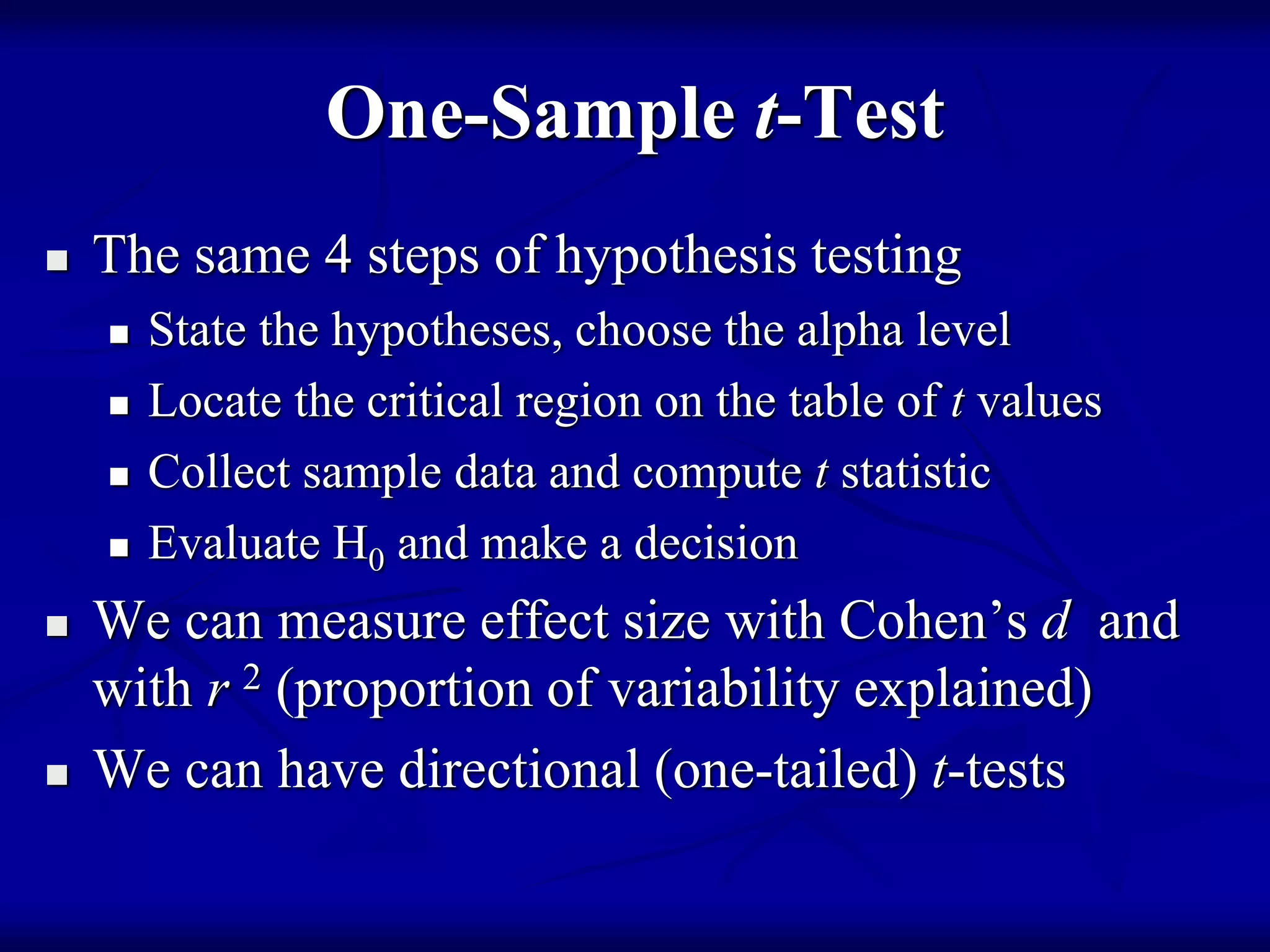
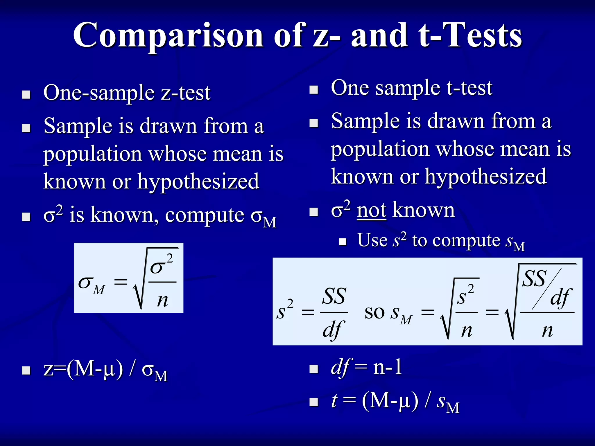
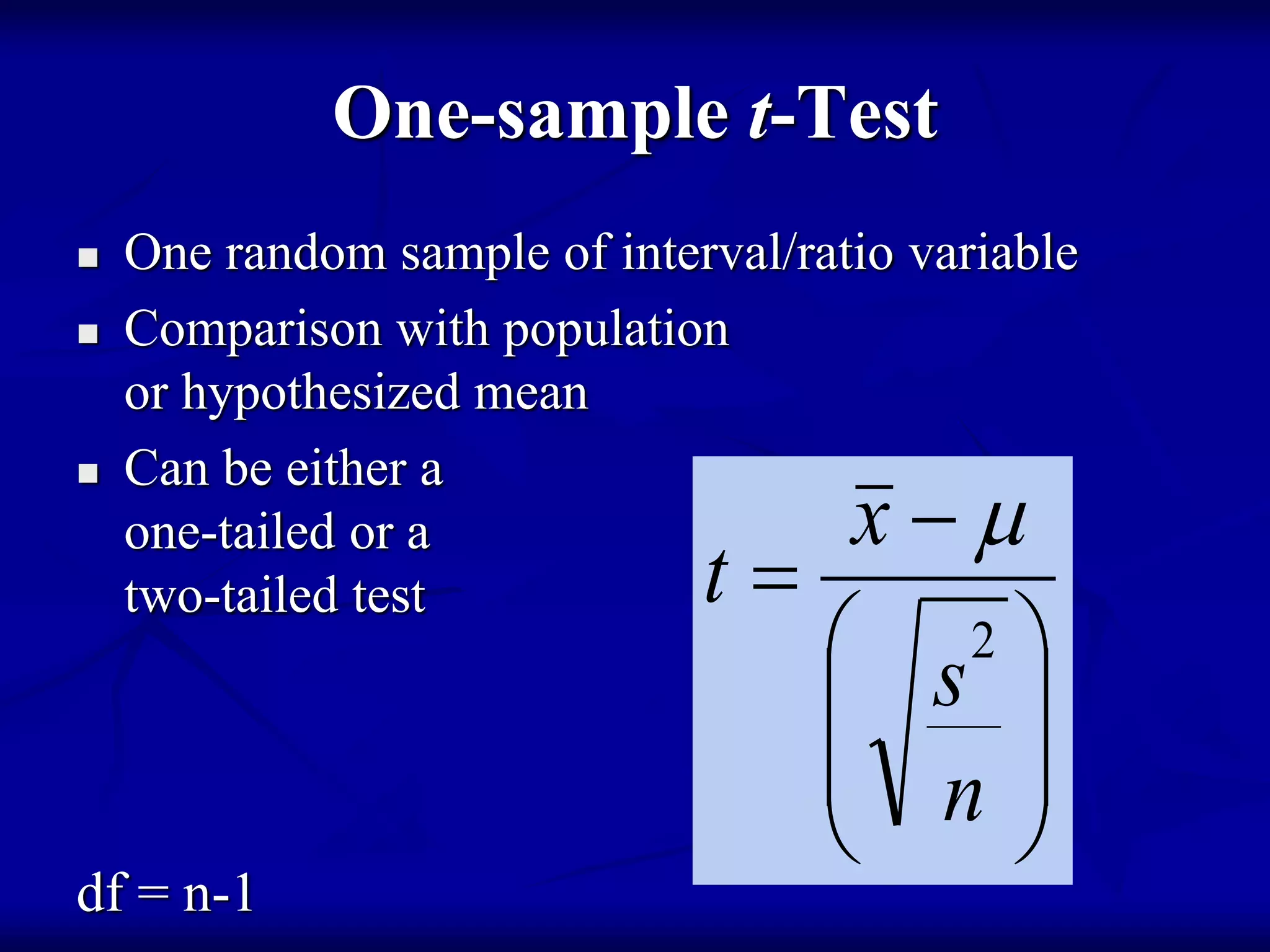
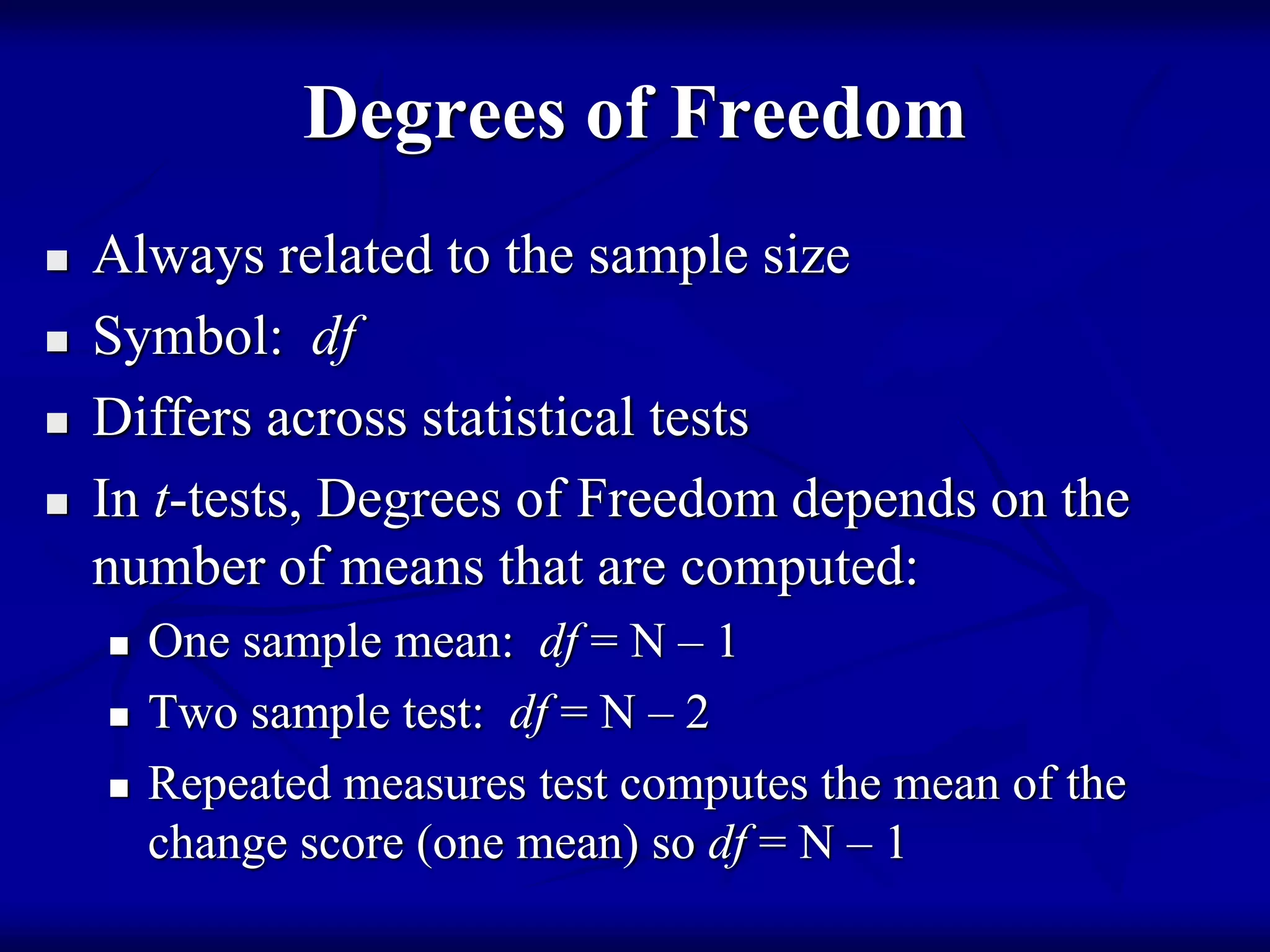
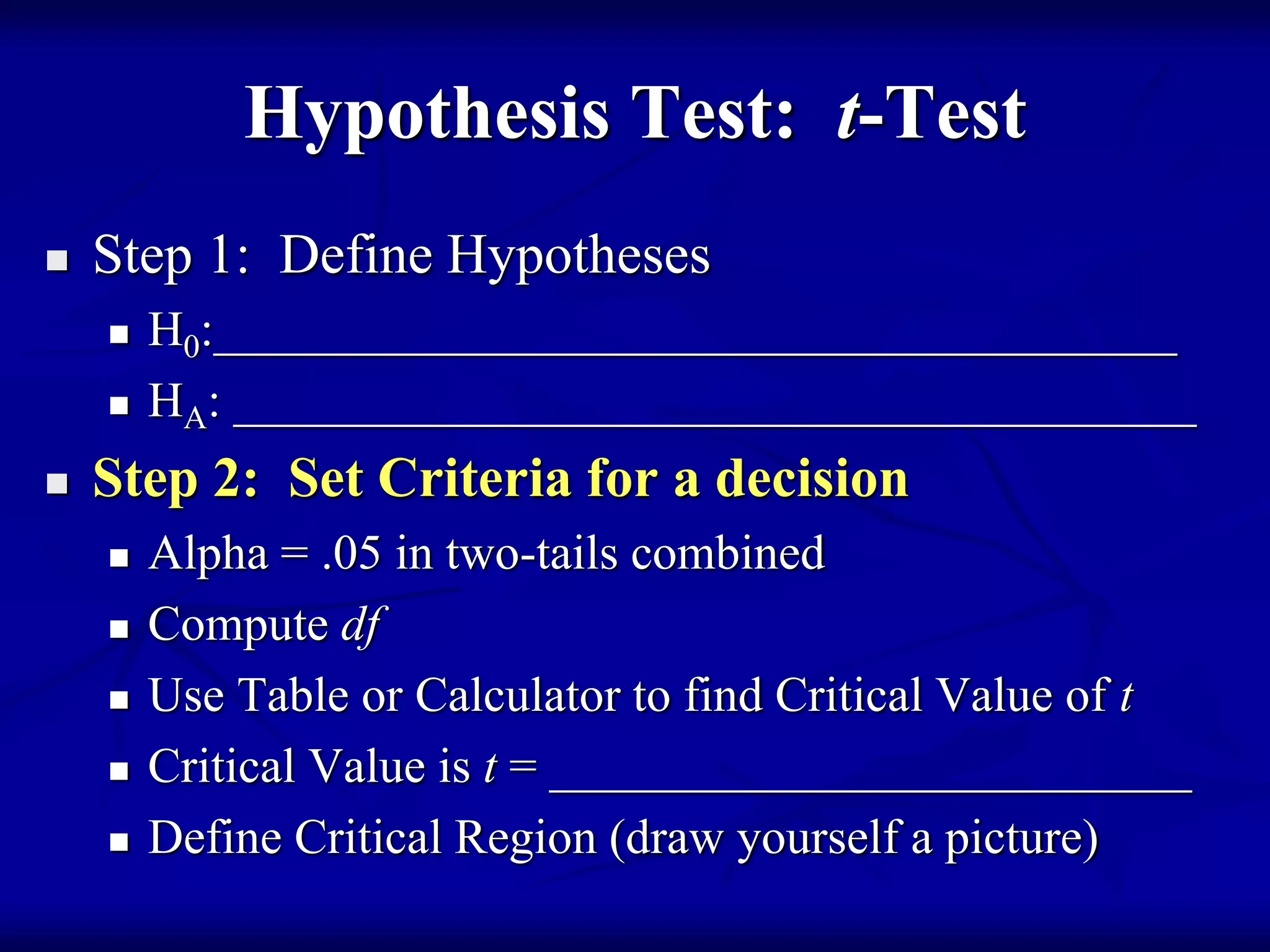
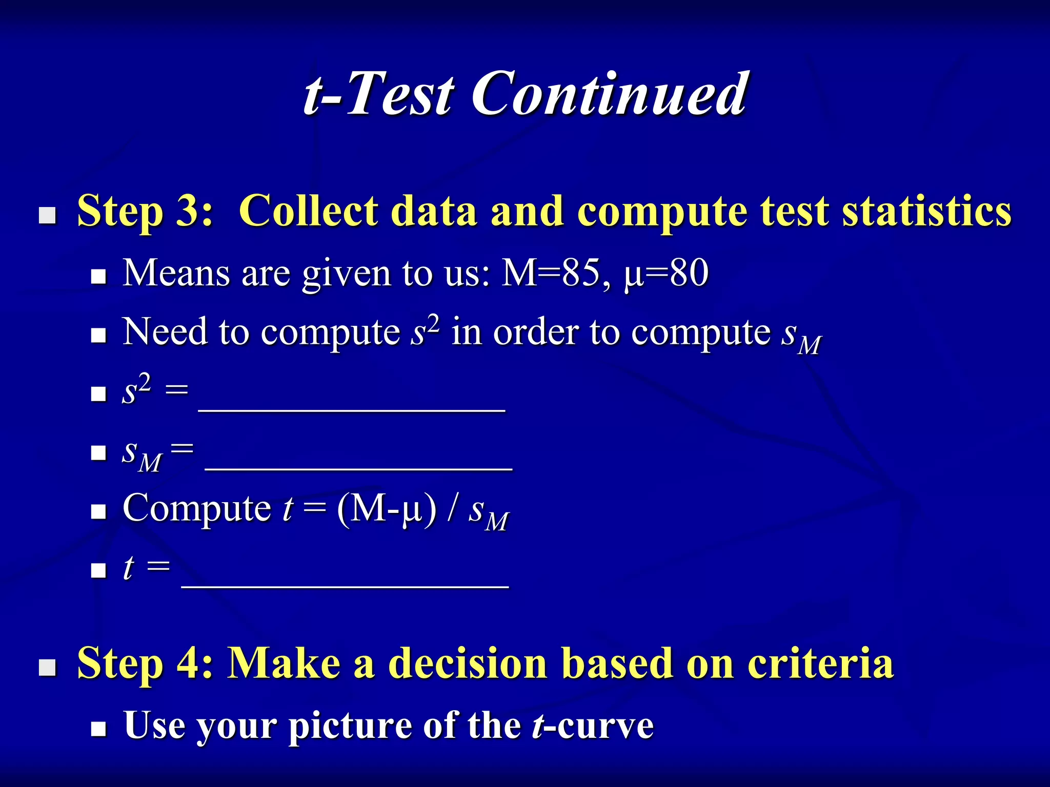
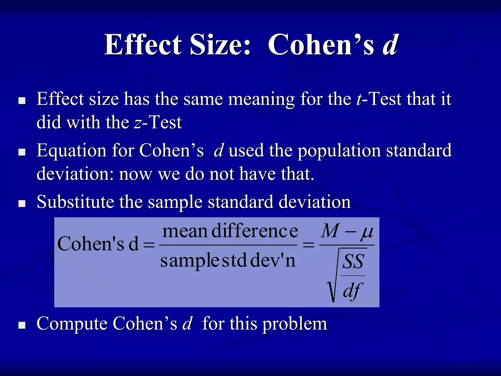
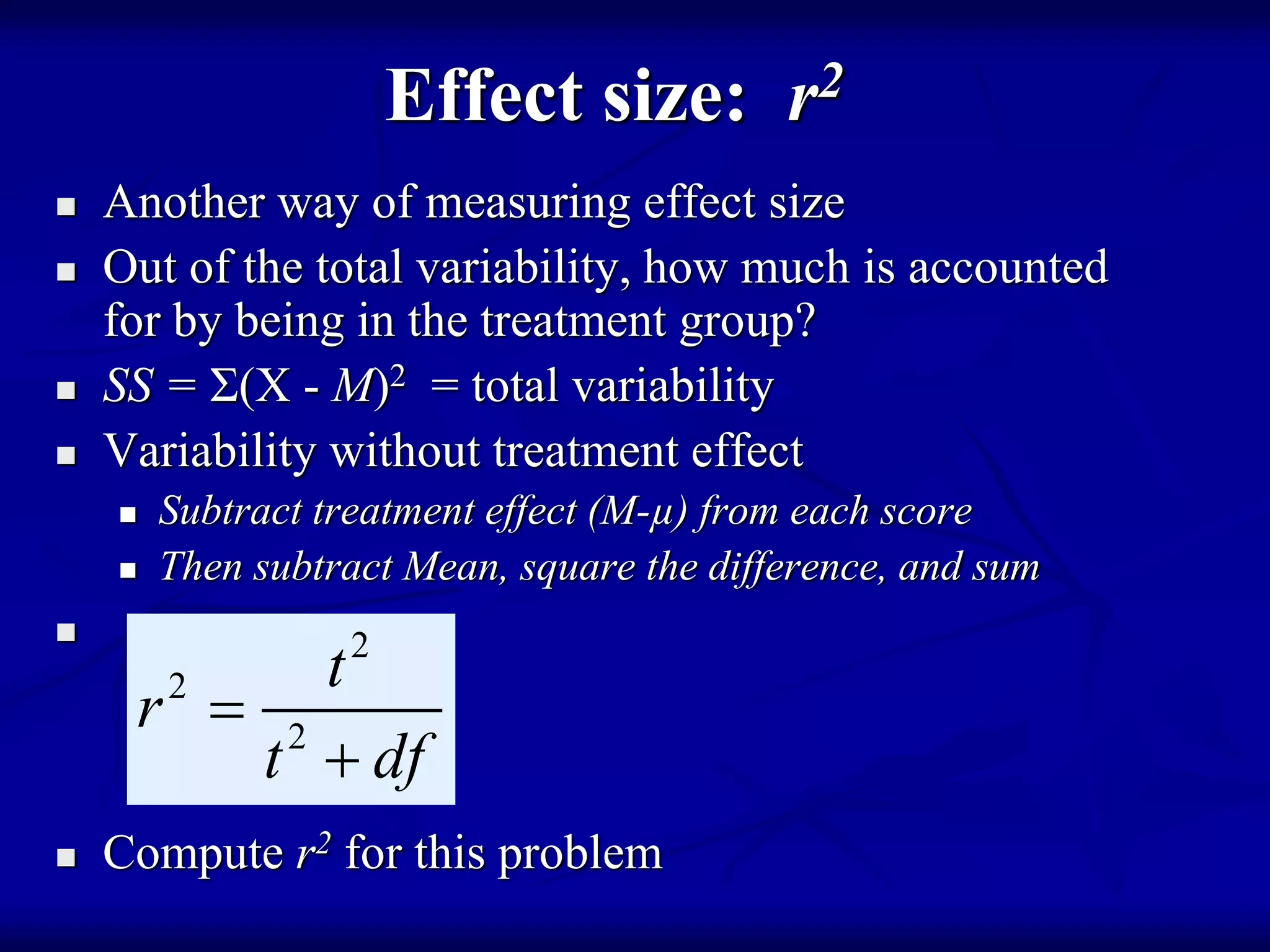
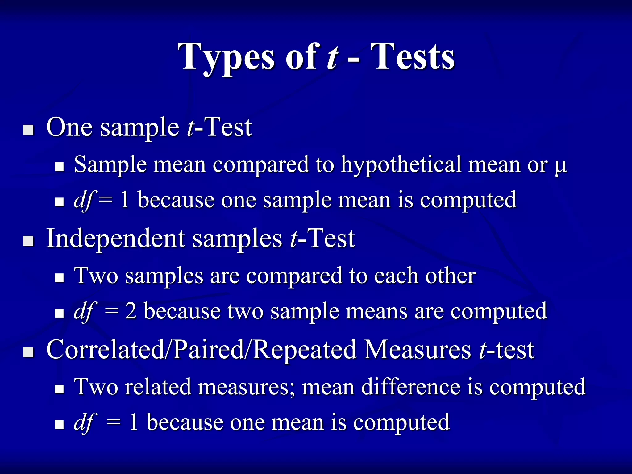
t-Tests give us more options
Inferential
Statistics
What we know already:
 Frequency distributions shown in graphs
 Summarizing data sets
 Central tendency (mean, median, mode)
 Variability (variance and standard deviation)
 Central Limit Theorem
 Sample means are normally distributed
 If n > 30 or population is normally distributed
 Hypothesis Testing basics
 Null hypothesis & critical region defined
 Sample data used to make a decision
Bad news:
“The shortcoming of using a z-score as an
inferential statistic is that the z-score formula
requires more information than is usually
available.”
“Specifically, a z-score requires that we know
the value of the population standard deviation
(or variance). In most situations, however,
the standard deviation for the population is
not known.”
One-Sample t-Test
 We want to compare a single sample to a
population mean, or a hypothetical mean
 We don’t know σ2 so we use s2, the Sample Variance
 We have an estimated standard error, sM
 We use sM to compute t
 t is similar to z in shape: bell curve
 It is shorter in the center, and the tails have more area
 There is more than one t curve
 The curve is determined by M, s2, and df
 Degrees of freedom, df is related to sample size
Distribution of the t statistic for different values of degrees of freedom are
compared to a normal z-score distribution. Like the normal distribution, t
distributions are bell-shaped and symmetrical and have a mean of zero. However, t
distributions have more variability, indicated by the flatter and more spread-out
shape. The larger the value of df is, the more closely the t distribution approximates
a normal distribution.
One-Sample t-Test
 The same 4 steps of hypothesis testing
 State the hypotheses, choose the alpha level
 Locate the critical region on the table of t values
 Collect sample data and compute t statistic
 Evaluate H0 and make a decision
 We can measure effect size with Cohen’s d and
with r 2 (proportion of variability explained)
 We can have directional (one-tailed) t-tests
Comparison of z- and t-Tests
 One-sample z-test
 Sample is drawn from a
population whose mean is
known or hypothesized
 σ2 is known, compute σM
 z=(M-µ) / σM
 One sample t-test
 Sample is drawn from a
population whose mean is
known or hypothesized
 σ2 not known
 Use s2 to compute sM
 df = n-1
 t = (M-µ) / sM
2
M
n

  2
2
so M
SS
SS s df
s s
df n n
  
One-sample t-Test
 One random sample of interval/ratio variable
 Comparison with population
or hypothesized mean
 Can be either a
one-tailed or a
two-tailed test
df = n-1










n
s
x
t
2

Degrees of Freedom
 Always related to the sample size
 Symbol: df
 Differs across statistical tests
 In t-tests, Degrees of Freedom depends on the
number of means that are computed:
 One sample mean: df = N – 1
 Two sample test: df = N – 2
 Repeated measures test computes the mean of the
change score (one mean) so df = N – 1
Sample Problem
A group of telemarketers averaged 80 sales per day.
A sample of n=16 people were randomly chosen for
training on a new technique. After training, the
sample averages 85 sales per day, with SS=60.
Does the sample provide sufficient evidence to
conclude that the training leads to higher levels of
sales?
THINK FIRST
 We cannot draw the population distribution,
because we do not know its standard deviation.
 We can draw the distribution of sales scores
(the scores of the 16 people) because we know the
mean and standard deviation of the sample.
 So: draw the curve representing the sample of
sales scores after training.
 What range contains about 95% of scores?
 Does it include the pre-training mean of 80?
Hypothesis Test: t-Test
 Step 1: Define Hypotheses
 H0:_______________________________________
 HA: _______________________________________
 Step 2: Set Criteria for a decision
 Alpha = .05 in two-tails combined
 Compute df
 Use Table or Calculator to find Critical Value of t
 Critical Value is t = __________________________
 Define Critical Region (draw yourself a picture)
t-Test Continued
 Step 3: Collect data and compute test statistics
 Means are given to us: M=85, µ=80
 Need to compute s2 in order to compute sM
 s2 = _______________
 sM = _______________
 Compute t = (M-µ) / sM
 t = ________________
 Step 4: Make a decision based on criteria
 Use your picture of the t-curve
Effect Size: Cohen’s d
 Effect size has the same meaning for the t-Test that it
did with the z-Test
 Equation for Cohen’s d used the population standard
deviation: now we do not have that.
 Substitute the sample standard deviation
 Compute Cohen’s d for this problem
df
SS
M 

ndev'stdsample
differencemean
dsCohen'
Effect size: r2
 Another way of measuring effect size
 Out of the total variability, how much is accounted
for by being in the treatment group?
 SS = Σ(X - M)2 = total variability
 Variability without treatment effect
 Subtract treatment effect (M-µ) from each score
 Then subtract Mean, square the difference, and sum

 Compute r2 for this problem
2
2
2
t
r
t df


How to Write Results
1. First sentence: What question was tested? Can
be a statement or a question.
2. Procedure / sample: How was the test done?
Who was tested?
3. What were the results? Report sample statistics
(M and sM), the test statistic (t) and its df,
the significance (p), and decision.
4. If significant, report effect size
5. Close with a summary sentence
Sample Narrative
A sample of 16 telemarketers received special
training. After training, their average daily sales
(M = 85, s = 2) were significantly higher than the
pre-training average of 80 for all the telemarketers
(t(15) = 10, p < .05). The effect size, measured
by Cohen’s d, is quite large (d = 2.5).
Approximately 87% of the variability is accounted
for by the training (r2 = .8695). The sales training
produced a significant and sizable difference,
leading to an increase in sales for the firm.
Types of t - Tests
 One sample t-Test
 Sample mean compared to hypothetical mean or μ
 df = 1 because one sample mean is computed
 Independent samples t-Test
 Two samples are compared to each other
 df = 2 because two sample means are computed
 Correlated/Paired/Repeated Measures t-test
 Two related measures; mean difference is computed
 df = 1 because one mean is computed
Basic dynamic of all of our tests
 They will involve a ratio (a fraction)
 The numerator (top) will measure variability
between group(s)
 The denominator (bottom) will measure the
variability that is due to random chance
 “Difference on the top, and error on the bottom”
Statz Rappers

Introduction to the t test

  • 1.
    t-Tests give usmore options Inferential Statistics
  • 2.
    What we knowalready:  Frequency distributions shown in graphs  Summarizing data sets  Central tendency (mean, median, mode)  Variability (variance and standard deviation)  Central Limit Theorem  Sample means are normally distributed  If n > 30 or population is normally distributed  Hypothesis Testing basics  Null hypothesis & critical region defined  Sample data used to make a decision
  • 3.
    Bad news: “The shortcomingof using a z-score as an inferential statistic is that the z-score formula requires more information than is usually available.” “Specifically, a z-score requires that we know the value of the population standard deviation (or variance). In most situations, however, the standard deviation for the population is not known.”
  • 4.
    One-Sample t-Test  Wewant to compare a single sample to a population mean, or a hypothetical mean  We don’t know σ2 so we use s2, the Sample Variance  We have an estimated standard error, sM  We use sM to compute t  t is similar to z in shape: bell curve  It is shorter in the center, and the tails have more area  There is more than one t curve  The curve is determined by M, s2, and df  Degrees of freedom, df is related to sample size
  • 5.
    Distribution of thet statistic for different values of degrees of freedom are compared to a normal z-score distribution. Like the normal distribution, t distributions are bell-shaped and symmetrical and have a mean of zero. However, t distributions have more variability, indicated by the flatter and more spread-out shape. The larger the value of df is, the more closely the t distribution approximates a normal distribution.
  • 6.
    One-Sample t-Test  Thesame 4 steps of hypothesis testing  State the hypotheses, choose the alpha level  Locate the critical region on the table of t values  Collect sample data and compute t statistic  Evaluate H0 and make a decision  We can measure effect size with Cohen’s d and with r 2 (proportion of variability explained)  We can have directional (one-tailed) t-tests
  • 7.
    Comparison of z-and t-Tests  One-sample z-test  Sample is drawn from a population whose mean is known or hypothesized  σ2 is known, compute σM  z=(M-µ) / σM  One sample t-test  Sample is drawn from a population whose mean is known or hypothesized  σ2 not known  Use s2 to compute sM  df = n-1  t = (M-µ) / sM 2 M n    2 2 so M SS SS s df s s df n n   
  • 8.
    One-sample t-Test  Onerandom sample of interval/ratio variable  Comparison with population or hypothesized mean  Can be either a one-tailed or a two-tailed test df = n-1           n s x t 2 
  • 9.
    Degrees of Freedom Always related to the sample size  Symbol: df  Differs across statistical tests  In t-tests, Degrees of Freedom depends on the number of means that are computed:  One sample mean: df = N – 1  Two sample test: df = N – 2  Repeated measures test computes the mean of the change score (one mean) so df = N – 1
  • 10.
    Sample Problem A groupof telemarketers averaged 80 sales per day. A sample of n=16 people were randomly chosen for training on a new technique. After training, the sample averages 85 sales per day, with SS=60. Does the sample provide sufficient evidence to conclude that the training leads to higher levels of sales?
  • 11.
    THINK FIRST  Wecannot draw the population distribution, because we do not know its standard deviation.  We can draw the distribution of sales scores (the scores of the 16 people) because we know the mean and standard deviation of the sample.  So: draw the curve representing the sample of sales scores after training.  What range contains about 95% of scores?  Does it include the pre-training mean of 80?
  • 12.
    Hypothesis Test: t-Test Step 1: Define Hypotheses  H0:_______________________________________  HA: _______________________________________  Step 2: Set Criteria for a decision  Alpha = .05 in two-tails combined  Compute df  Use Table or Calculator to find Critical Value of t  Critical Value is t = __________________________  Define Critical Region (draw yourself a picture)
  • 13.
    t-Test Continued  Step3: Collect data and compute test statistics  Means are given to us: M=85, µ=80  Need to compute s2 in order to compute sM  s2 = _______________  sM = _______________  Compute t = (M-µ) / sM  t = ________________  Step 4: Make a decision based on criteria  Use your picture of the t-curve
  • 14.
    Effect Size: Cohen’sd  Effect size has the same meaning for the t-Test that it did with the z-Test  Equation for Cohen’s d used the population standard deviation: now we do not have that.  Substitute the sample standard deviation  Compute Cohen’s d for this problem df SS M   ndev'stdsample differencemean dsCohen'
  • 15.
    Effect size: r2 Another way of measuring effect size  Out of the total variability, how much is accounted for by being in the treatment group?  SS = Σ(X - M)2 = total variability  Variability without treatment effect  Subtract treatment effect (M-µ) from each score  Then subtract Mean, square the difference, and sum   Compute r2 for this problem 2 2 2 t r t df  
  • 16.
    How to WriteResults 1. First sentence: What question was tested? Can be a statement or a question. 2. Procedure / sample: How was the test done? Who was tested? 3. What were the results? Report sample statistics (M and sM), the test statistic (t) and its df, the significance (p), and decision. 4. If significant, report effect size 5. Close with a summary sentence
  • 17.
    Sample Narrative A sampleof 16 telemarketers received special training. After training, their average daily sales (M = 85, s = 2) were significantly higher than the pre-training average of 80 for all the telemarketers (t(15) = 10, p < .05). The effect size, measured by Cohen’s d, is quite large (d = 2.5). Approximately 87% of the variability is accounted for by the training (r2 = .8695). The sales training produced a significant and sizable difference, leading to an increase in sales for the firm.
  • 18.
    Types of t- Tests  One sample t-Test  Sample mean compared to hypothetical mean or μ  df = 1 because one sample mean is computed  Independent samples t-Test  Two samples are compared to each other  df = 2 because two sample means are computed  Correlated/Paired/Repeated Measures t-test  Two related measures; mean difference is computed  df = 1 because one mean is computed
  • 19.
    Basic dynamic ofall of our tests  They will involve a ratio (a fraction)  The numerator (top) will measure variability between group(s)  The denominator (bottom) will measure the variability that is due to random chance  “Difference on the top, and error on the bottom”
  • 20.