Chapter six Bio (1).pptx for students and others

University of Gondar
College of medicine and health
science
Department of Epidemiology and Biostatistics
Chapter Seven: Statistical Inference
By: Berhanie Addis (MSc.)
Email: berhanieaddis36@gmail.com

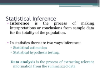
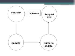
Statistical Inference
• Inference is the process of making
interpretations or conclusions from sample data
for the totality of the population.
• In statistics there are two ways inference:
▫ Statistical estimation
▫ Statistical hypothesis testing.
Data analysis is the process of extracting relevant
information from the summarized data

Population
Sample Numeric
al data
Analyzed
Data
Inference

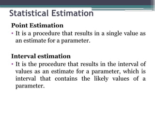
Statistical Estimation
Point Estimation
• It is a procedure that results in a single value as
an estimate for a parameter.
Interval estimation
• It is the procedure that results in the interval of
values as an estimate for a parameter, which is
interval that contains the likely values of a
parameter.

Definitions
• Confidence Interval: An interval estimate
with a specific level of confidence
• Confidence Level: The percent of the time
that the true value will lie in the interval
estimate given.
• Consistent Estimator: An estimator which
gets closer to the value of the parameter as the
sample size increases.

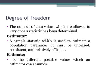
Degree of freedom
• The number of data values which are allowed to
vary once a statistic has been determined.
Estimator:
• A sample statistic which is used to estimate a
population parameter. It must be unbiased,
consistent, and relatively efficient.
Estimate:
• Is the different possible values which an
estimator can assumes.

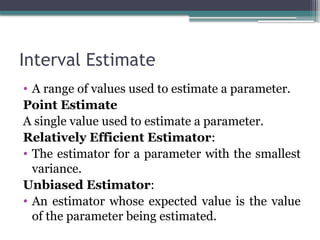
Interval Estimate
• A range of values used to estimate a parameter.
Point Estimate
A single value used to estimate a parameter.
Relatively Efficient Estimator:
• The estimator for a parameter with the smallest
variance.
Unbiased Estimator:
• An estimator whose expected value is the value
of the parameter being estimated.

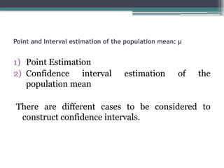
Point and Interval estimation of the population mean: µ
1) Point Estimation
2) Confidence interval estimation of the
population mean
There are different cases to be considered to
construct confidence intervals.

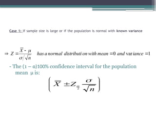
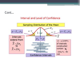
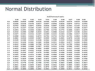
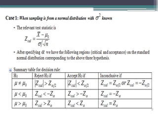
Case 1: If sample size is large or if the population is normal with known variance
- The (1 – α)100% confidence interval for the population
mean µ is:
1
var
0 



 iance
and
mean
with
on
distributi
normal
a
has
n
X
Z









n
Z
X


2

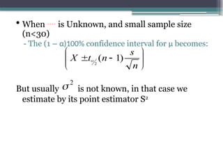
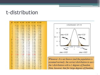
• When  is Unknown, and small sample size
(n<30)
- The (1 – α)100% confidence interval for µ becomes:
But usually is not known, in that case we
estimate by its point estimator S2








n
s
n
t
X )
1
(
2

2


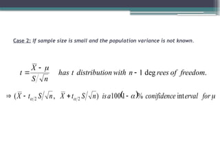
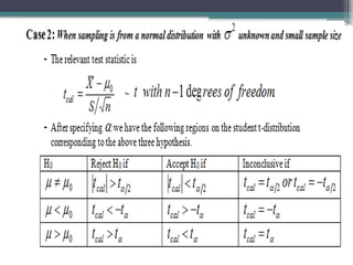
Case 2: If sample size is small and the population variance is not known.
.
deg
1 freedom
of
rees
n
with
on
distributi
t
has
n
S
X
t 



  


 for
erval
e
conifidenc
a
is
n
S
t
X
n
S
t
X int
%
1
100
)
,
( 2
2 




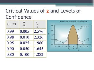
0.99 0.005 2.576
0.98 0.010 2.326
0.95 0.025 1.960
0.90 0.050 1.645
0.80 0.100 1.282
( )
1 

2
z
2
Critical Values of z and Levels of
Confidence
5
4
3
2
1
0
-1
-2
-3
-4
-5
0.4
0.3
0.2
0.1
0.0
Z
f(z)
Stand ard Norm al Distribution
z
2
( )
1  
 z
2

2

2

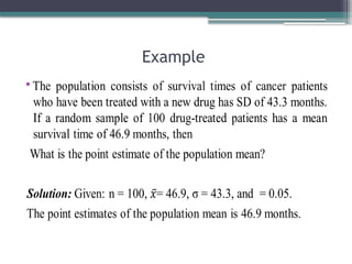
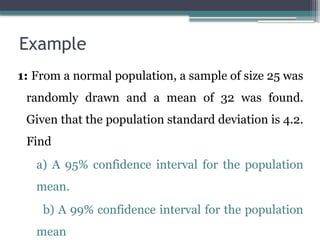
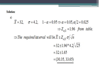
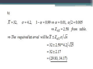
Example
1: From a normal population, a sample of size 25 was
randomly drawn and a mean of 32 was found.
Given that the population standard deviation is 4.2.
Find
a) A 95% confidence interval for the population
mean.
b) A 99% confidence interval for the population
mean

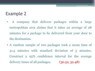
Example 2
• A company that delivers packages within a large
metropolitan area claims that it takes an average of 28
minutes for a package to be delivered from your door to
the destination.
• A random sample of 100 packages took a mean time of
31.5 minutes with standard deviation of 5 minutes.
Construct a 95% confidence interval for the average
delivery times of all packages. (30.52, 32.48)

Example 3
• A stock market analyst wants to estimate the
average return on a certain stock. A random
sample of 15 days yields an average (annualized)
return of 10.37% and a standard deviation of
3.5%. Assuming a normal population of returns,
give a 95% confidence interval for the average
return on this stock. (8.43,. 12.31))

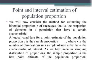
Point and interval estimation of
population proportion
• We will now consider the method for estimating the
binomial proportion p of successes, that is, the proportion
of elements in a population that have a certain
characteristic.
A logical candidate for a point estimate of the population
proportion p is the sample proportion , where x is the
number of observations in a sample of size n that have the
characteristic of interest. As we have seen in sampling
distribution of proportions, the sample proportion is the
best point estimate of the population proportion.

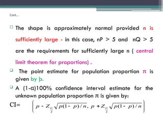
Cont…
 The shape is approximately normal provided n is
sufficiently large - in this case, nP > 5 and nQ > 5
are the requirements for sufficiently large n ( central
limit theorem for proportions) .
 The point estimate for population proportion π is
given by þ.
 A (1-α)100% confidence interval estimate for the
unknown population proportion π is given by:
CI= 










 n
p
p
Z
p
n
p
p
Z
p /
)
1
(
,
/
)
1
(
2
2



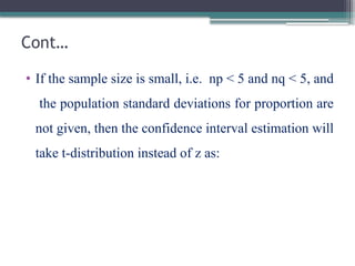
Cont…
• If the sample size is small, i.e. np < 5 and nq < 5, and
the population standard deviations for proportion are
not given, then the confidence interval estimation will
take t-distribution instead of z as:

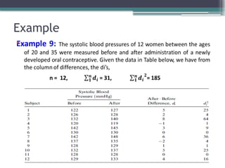
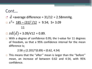
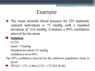
Example
The mean diastolic blood pressure for 225 randomly
selected individuals is 75 mmHg with a standard
deviation of 12.0 mmHg. Construct a 95% confidence
interval for the mean
Solution
n=225
mean =75mmhg
Standard deviation=12 mmHg
confidence level 95%
The 95% confidence interval for the unknown population mean is
given
95%CI = (75 ±1.96x12/15) = (73.432,76.56)

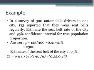
Example
• In a survey of 300 automobile drivers in one
city, 123 reported that they wear seat belts
regularly. Estimate the seat belt rate of the city
and 95% confidence interval for true population
proportion.
• Answer : p= 123/300 =0.41=41%
n=300,
Estimate of the seat belt of the city at 95%
CI = p ± z ×(√p(1-p) /n) =(0.35,0.47)

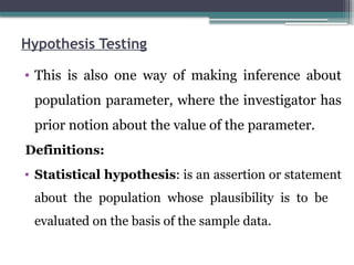
Hypothesis Testing
• This is also one way of making inference about
population parameter, where the investigator has
prior notion about the value of the parameter.
Definitions:
• Statistical hypothesis: is an assertion or statement
about the population whose plausibility is to be
evaluated on the basis of the sample data.

Test statistic: is a statistics whose value serves to determine whether to reject or accept the hypothesis to be tested. It is a random variable.
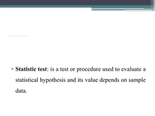
• Statistic test: is a test or procedure used to evaluate a
statistical hypothesis and its value depends on sample
data.

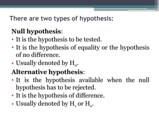
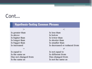
There are two types of hypothesis:
Null hypothesis:
• It is the hypothesis to be tested.
• It is the hypothesis of equality or the hypothesis
of no difference.
• Usually denoted by H0.
Alternative hypothesis:
• It is the hypothesis available when the null
hypothesis has to be rejected.
• It is the hypothesis of difference.
• Usually denoted by H1 or Ha.

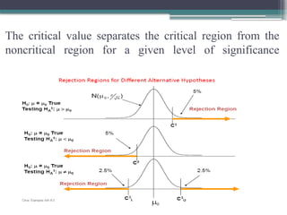
The critical value separates the critical region from the
noncritical region for a given level of significance

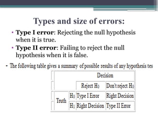
Types and size of errors:
• Type I error: Rejecting the null hypothesis
when it is true.
• Type II error: Failing to reject the null
hypothesis when it is false.

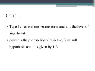
Cont…
• Type I error is more serious error and it is the level of
significant
• power is the probability of rejecting false null
hypothesis and it is given by 1-β

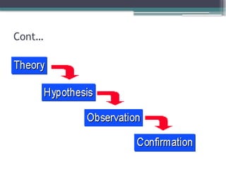
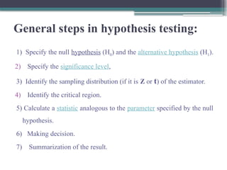
General steps in hypothesis testing:
1) Specify the null hypothesis (H0) and the alternative hypothesis (H1).
2) Specify the significance level,
3) Identify the sampling distribution (if it is Z or t) of the estimator.
4) Identify the critical region.
5) Calculate a statistic analogous to the parameter specified by the null
hypothesis.
6) Making decision.
7) Summarization of the result.

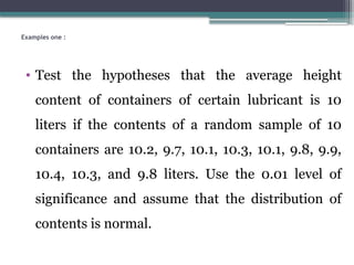
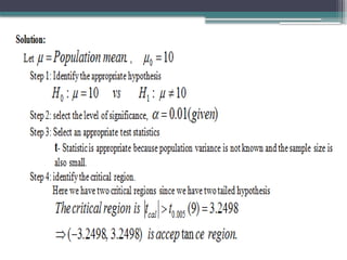
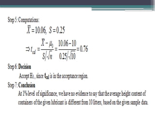
Hypothesis testing about the population mean, :

Examples one :
• Test the hypotheses that the average height
content of containers of certain lubricant is 10
liters if the contents of a random sample of 10
containers are 10.2, 9.7, 10.1, 10.3, 10.1, 9.8, 9.9,
10.4, 10.3, and 9.8 liters. Use the 0.01 level of
significance and assume that the distribution of
contents is normal.

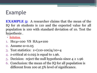
Example
EXAMPLE 5: A researcher claims that the mean of the
IQ for 16 students is 110 and the expected value for all
population is 100 with standard deviation of 10. Test the
hypothesis .
• Solution
1. Ho:µ=100 VS HA:µ≠100
2. Assume α=0.05
3. Test statistics: z=(110-100)4/10=4
4. z-critical at 0.025 is equal to 1.96.
5. Decision: reject the null hypothesis since 4 ≥ 1.96
6. Conclusion: the mean of the IQ for all population is
different from 100 at 5% level of significance.

Example
In the study of childhood abuse in psychiatry patients, brown found
that 166 in a sample of 947 patients reported histories of physical or
sexual abuse.
a) constructs 95% confidence interval
b) test the hypothesis that the true population proportion
is 30%?
• Solution (a)
▫ The 95% CI for P is given by
]
2
.
0
;
151
.
0
[
0124
.
0
96
.
1
175
.
0
947
825
.
0
175
.
0
96
.
1
175
.
0
)
1
(
2











n
p
p
z
p 

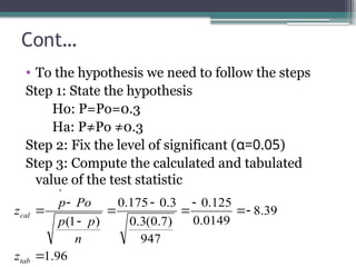
Cont…
• To the hypothesis we need to follow the steps
Step 1: State the hypothesis
Ho: P=Po=0.3
Ha: P≠Po ≠0.3
Step 2: Fix the level of significant (α=0.05)
Step 3: Compute the calculated and tabulated
value of the test statistic
96
.
1
39
.
8
0149
.
0
125
.
0
947
)
7
.
0
(
3
.
0
3
.
0
175
.
0
)
1
(











tab
cal
z
n
p
p
Po
p
z

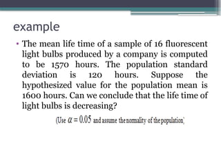
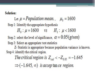
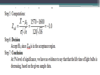
example
• The mean life time of a sample of 16 fluorescent
light bulbs produced by a company is computed
to be 1570 hours. The population standard
deviation is 120 hours. Suppose the
hypothesized value for the population mean is
1600 hours. Can we conclude that the life time of
light bulbs is decreasing?

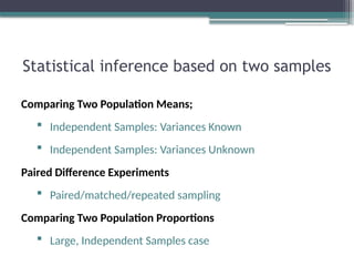
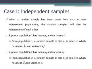
Statistical inference based on two samples
Comparing Two Population Means;
 Independent Samples: Variances Known
 Independent Samples: Variances Unknown
Paired Difference Experiments
 Paired/matched/repeated sampling
Comparing Two Population Proportions
 Large, Independent Samples case

Case I: independent samples
•

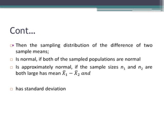
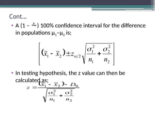
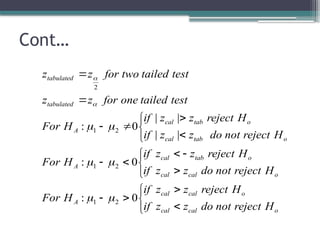
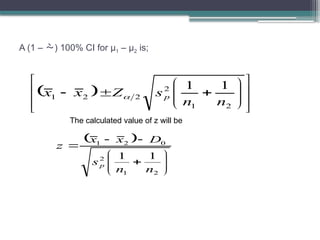
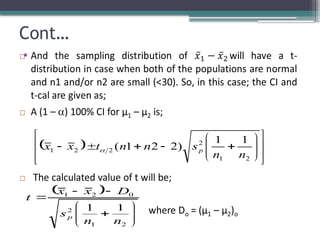
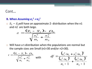
Cont…
• A (1 – ) 100% confidence interval for the difference
in populations µ1–µ2 is;
• In testing hypothesis, the z value can then be
calculated as;
 











2
2
2
1
2
1
2
2
1
n
n
z
x
x



 
2
2
2
1
2
1
0
2
1
n
n
D
x
x
z







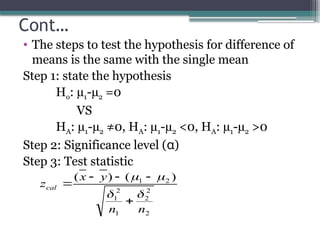
Cont…
• The steps to test the hypothesis for difference of
means is the same with the single mean
Step 1: state the hypothesis
Ho: µ1-µ2 =0
VS
HA: µ1-µ2 ≠0, HA: µ1-µ2 <0, HA: µ1-µ2 >0
Step 2: Significance level (α)
Step 3: Test statistic
2
2
2
1
2
1
2
1 )
(
)
(
n
n
y
x
zcal










Cont…
























o
cal
cal
o
cal
cal
A
o
cal
cal
o
tab
cal
A
o
tab
cal
o
tab
cal
A
tabulated
tabulated
H
reject
not
do
z
z
if
H
reject
z
z
if
H
For
H
reject
not
do
z
z
if
H
reject
z
z
if
H
For
H
reject
not
do
z
z
if
H
reject
z
z
if
H
For
test
tailed
one
for
z
z
test
tailed
two
for
z
z
0
:
0
:
|
|
|
|
0
:
2
1
2
1
2
1
2









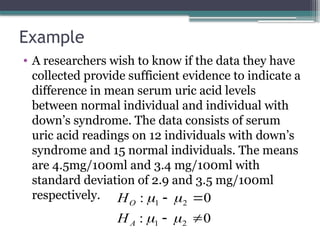
Example
• A researchers wish to know if the data they have
collected provide sufficient evidence to indicate a
difference in mean serum uric acid levels
between normal individual and individual with
down’s syndrome. The data consists of serum
uric acid readings on 12 individuals with down’s
syndrome and 15 normal individuals. The means
are 4.5mg/100ml and 3.4 mg/100ml with
standard deviation of 2.9 and 3.5 mg/100ml
respectively.
0
:
0
:
2
1
2
1








A
O
H
H

Cont…
96
.
1
33
.
5
23
.
1
6
.
1
5178
.
1
6
.
1
15
5
.
3
12
9
.
2
0
)
4
.
3
3
.
4
(
)
(
)
(
025
.
0
2
2
2
2
2
2
1
2
1
2
1














z
z
n
n
y
x
zcal






Independent sample with unknown variance
•

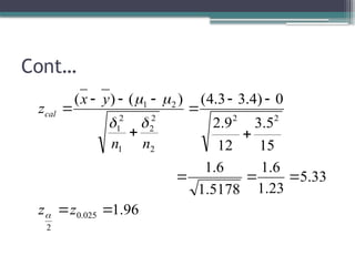
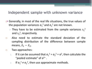
Cont…
A. Assume that the unknown variances; σ1
2
= σ2
2
= σ2
The pooled estimate of σ2
is the weighted average of
the two sample variances, s1
2
and s2
2
The pooled estimate of σ2
is denoted by sp
The estimate of the population standard deviation of
the sampling distribution is;
   
2
1
1
2
1
2
2
2
2
1
1
2






n
n
s
n
s
n
sp










 
2
1
2 1
1
2
1
n
n
sp
x
x

A (1 – ) 100% CI for µ1 – µ2 is;
 



















2
1
2
2
2
1
1
1
n
n
s
Z
x
x p

The calculated value of z will be
 












2
1
2
0
2
1
1
1
n
n
s
D
x
x
z
p

Cont…
•
 





















2
1
2
2
2
1
1
1
)
2
2
1
(
n
n
s
n
n
t
x
x p

 












2
1
2
0
2
1
1
1
n
n
s
D
x
x
t
p

Cont…
•
 
2
2
2
1
2
1
0
2
1
n
s
n
s
D
x
x
z




 
2
2
2
1
2
1
0
2
1
n
s
n
s
D
x
x
t



  
   
1
1 2
2
2
2
2
1
2
1
2
1
2
2
2
2
1
2
1





n
/n
s
n
/n
s
/n
s
/n
s
df

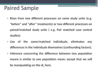
Paired Sample
• Rises from two different processes on same study units (e.g.
"before” and “after” treatments) or two different processes on
paired/matched study units ( e.g. Pair matched case control
studies).
• Use of the same/matched individuals, eliminates any
differences in the individuals themselves (confounding factors).
• Inference concerning the difference between two population
means is similar to one population mean; except that we will
be manipulating on the dis here.

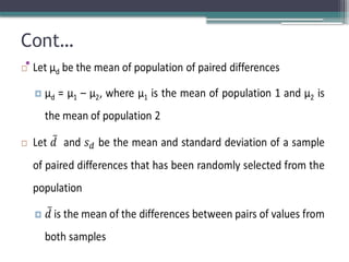
Cont…
• If the population of differences is normally distributed with
mean d
• A (1- )100% confidence interval for
µd = µ1 - µ2 is:
• Where for a sample of size n, t/2 is based on n – 1 degrees of
freedom.
• but Z-test can be used if the sample size is large
(n1=n2=n>30).






 
n
s
t
d d
/2

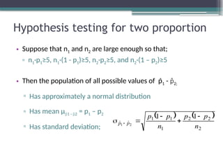
Hypothesis testing for two proportion
• Suppose that n1 and n2 are large enough so that;
▫ n1·p1≥5, n1·(1 - p1)≥5, n2·p2≥5, and n2·(1 – p2)≥5
• Then the population of all possible values of p̂1 - p̂2;
▫ Has approximately a normal distribution
▫ Has mean µ 1 - 2
p̂ p̂ = p1 – p2
▫ Has standard deviation;
   
2
2
2
1
1
1 1
1
2
1
n
p
p
n
p
p
p̂
p̂




 

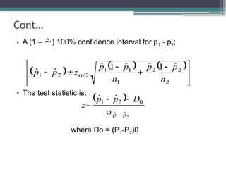
Cont…
• A (1 – ) 100% confidence interval for p1 - p2;
• The test statistic is;
where Do = (P1-P2)0
     







 



 
2
2
2
1
1
1
2
2
1
1
1
n
p̂
p̂
n
p̂
p̂
z
p̂
p̂
 
2
1
0
2
1
p̂
p̂
D
p̂
p̂
z=





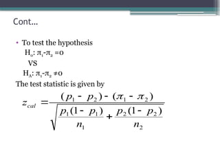
Cont…
• To test the hypothesis
Ho: π1-π2 =0
VS
HA: π1-π2 ≠0
The test statistic is given by
2
2
2
1
1
1
2
1
2
1
)
1
(
)
1
(
)
(
)
(
n
p
p
n
p
p
p
p
zcal










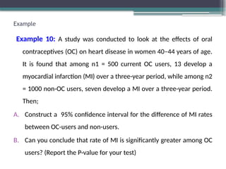
Example
Example 10: A study was conducted to look at the effects of oral
contraceptives (OC) on heart disease in women 40–44 years of age.
It is found that among n1 = 500 current OC users, 13 develop a
myocardial infarction (MI) over a three-year period, while among n2
= 1000 non-OC users, seven develop a MI over a three-year period.
Then;
A. Construct a 95% confidence interval for the difference of MI rates
between OC-users and non-users.
B. Can you conclude that rate of MI is significantly greater among OC
users? (Report the P-value for your test)

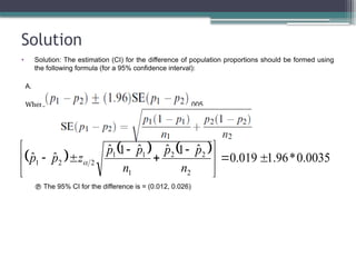
Solution
• Solution: The estimation (CI) for the difference of population proportions should be formed using
the following formula (for a 95% confidence interval):
A.
Where ≈ 0.005.
 The 95% CI for the difference is = (0.012, 0.026)
      0035
.
0
*
96
.
1
019
.
0
ˆ
1
ˆ
ˆ
1
ˆ
ˆ
ˆ
2
2
2
1
1
1
2
2
1 






 




n
p
p
n
p
p
z
p
p 

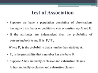
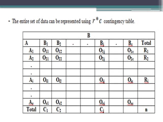
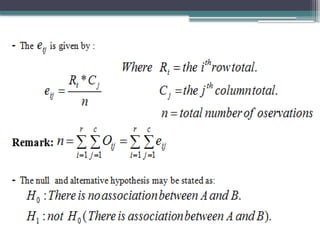
Test of Association
• Suppose we have a population consisting of observations
having two attributes or qualitative characteristics say A and B.
• If the attributes are independent then the probability of
possessing both A and B is PA*PB
Where PA is the probability that a number has attribute A.
• PB is the probability that a number has attribute B.
• Suppose A has mutually exclusive and exhaustive classes.
B has mutually exclusive and exhaustive classes

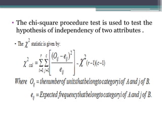
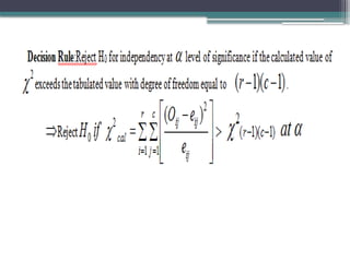
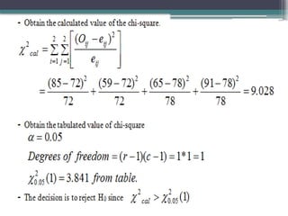
• The chi-square procedure test is used to test the
hypothesis of independency of two attributes .

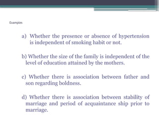
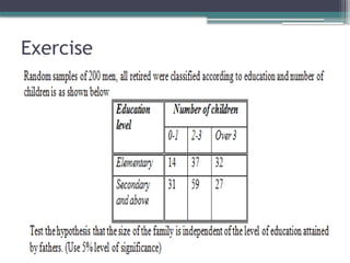
Examples
a) Whether the presence or absence of hypertension
is independent of smoking habit or not.
b) Whether the size of the family is independent of the
level of education attained by the mothers.
c) Whether there is association between father and
son regarding boldness.
d) Whether there is association between stability of
marriage and period of acquaintance ship prior to
marriage.

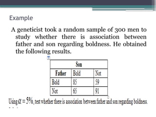
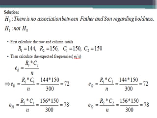
Example
A geneticist took a random sample of 300 men to
study whether there is association between
father and son regarding boldness. He obtained
the following results.

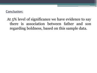
Conclusion:
At 5% level of significance we have evidence to say
there is association between father and son
regarding boldness, based on this sample data.

Chapter six Bio (1).pptx for students and others

More Related Content

Similar to Chapter six Bio (1).pptx for students and others

Recently uploaded

Chapter six Bio (1).pptx for students and others