


![Sampling Distribution of the Mean
Suppose we draw all possible samples of size n from a population of size N.
Suppose further that we compute a mean score for each sample. In this way, we create a sampling distribution
of the mean.
We know the following about the sampling distribution of the mean:
1. The mean of the sampling distribution (μx) is equal to the mean of the population (μ).
2. And the standard error of the sampling distribution (σx) is determined by the standard deviation of the
population (σ), the population size (N), and the sample size (n).
μx = μ
σx = [ σ / sqrt(n) ] * sqrt[ (N - n ) / (N - 1) ]
The factor sqrt[ (N - n ) / (N - 1) ] is called the finite population correction.
When the population size is very large relative to the sample size, the fpc is approximately equal to one; and the
standard error formula can be approximated by:
σx = σ / sqrt(n)
As a general rule, it is safe to use the approximate formula when the sample size is no bigger than 1/20 of the population size.](https://image.slidesharecdn.com/lesson7inferentialstatistics-200626230203/85/Inferential-Statistics-16-320.jpg)
![Sampling Distribution of the Proportion
Suppose we draw all possible samples of size n from a population of size N.
In a population of size N, suppose that the probability of the occurrence of an event (dubbed a "success") is P;
and the probability of the event's non-occurrence (dubbed a "failure") is Q.
From this population, suppose that we draw all possible samples of size n. And finally, within each sample,
suppose that we determine the proportion of successes p and failures q.
In this way, we create a sampling distribution of the proportion.
Results:
We find that the mean of the sampling distribution of the proportion (μp) is equal to the probability of success in
the population (P).
And the standard error of the sampling distribution (σp) is determined by the standard deviation of the
population (σ), the population size, and the sample size.
μp = P
σp = [ σ / sqrt(n) ] * sqrt[ (N - n ) / (N - 1) ]
σp = sqrt[ PQ/n ] * sqrt[ (N - n ) / (N - 1) ]
Or σp = sqrt[ PQ/n ] if finite correction is not applied.](https://image.slidesharecdn.com/lesson7inferentialstatistics-200626230203/85/Inferential-Statistics-17-320.jpg)


![T Distribution
It is a probability distribution that is used to estimate population parameters when:
1) The sample size is small or
2) When the population variance is unknown.
According to the central limit theorem, the sampling distribution of a statistic (like a sample mean) will follow a
normal distribution, as long as the sample size is sufficiently large. Therefore, when we know the standard
deviation of the population, we can compute a z-score, and use the normal distribution to evaluate probabilities
with the sample mean.
But sample sizes are sometimes small, and often we do not know the standard deviation of the population. And
we rely on the distribution of the t statistic (also known as the t score), whose values are given by:
t = [ x - μ ] / [ s / sqrt( n ) ]
where x is the sample mean, μ is the population mean, s is the standard deviation of the sample, and n is the
sample size.
The t distribution allows us to conduct statistical analyses on certain data sets that are not appropriate for
analysis, using the normal distribution](https://image.slidesharecdn.com/lesson7inferentialstatistics-200626230203/85/Inferential-Statistics-27-320.jpg)


![Estimation – Standard Error
The standard error is an estimate of the standard deviation of a statistic.
Standard Deviation of Sample Estimates: Statisticians use sample statistics to estimate population
parameters. Naturally, the value of a statistic may vary from one sample to the next. The variability of a
statistic is measured by its standard deviation.
The table below shows formulas for computing the standard deviation of statistics from simple random
samples.
Sample mean, x σx = σ / sqrt( n )
Sample proportion, p σp = sqrt [ P(1 - P) / n ]
Difference between means, x1 - x2 σx1-x2 = sqrt [ σ2
1 / n1 + σ2
2 / n2 ]
Note: In order to compute the standard deviation of a sample statistic, you must know the value of one or
more population parameters. For example, to compute the standard deviation of the sample mean (σx),
you need to know the variance of the population (σ).
What if we don’t know the population parameters?](https://image.slidesharecdn.com/lesson7inferentialstatistics-200626230203/85/Inferential-Statistics-36-320.jpg)
![Estimation – Standard Error
The standard error is an estimate of the standard deviation of a statistic.
Standard Error of Sample Estimates: Sadly, the values of population parameters are often unknown, making
it impossible to compute the standard deviation of a statistic. When this occurs, use the standard error.
The standard error is computed from known sample statistics. The table below shows how to compute the
standard error for simple random samples, assuming the population size is at least 20 times larger than the
sample size.
The equations for the standard error are identical to the equations for the standard deviation, except for
one thing - the standard error equations use statistics where the standard deviation equations use
parameters.
Sample mean, x SEx = s / sqrt( n )
Sample proportion, p SEp = sqrt [ p(1 - p) / n ]
Difference between means, x1 - x2 SEx1-x2 = sqrt [ s2
1 / n1 + s2
2 / n2 ]](https://image.slidesharecdn.com/lesson7inferentialstatistics-200626230203/85/Inferential-Statistics-37-320.jpg)


![Hypothesis Testing
Hypothesis Test for a Proportion:
- Compute the standard deviation (σ) of the sampling distribution: σ = sqrt[ P * ( 1 - P ) / n ]
where P is the hypothesized value of population proportion in the null hypothesis, and n is the sample size
- Test statistics: z = (p - P) / σ
where P is the hypothesized value of population proportion in the null hypothesis, p is the sample proportion,
and σ is the standard deviation of the sampling distribution.
Example 1:
The CEO of a large electric utility claims that 80 percent of his 1,000,000 customers are very satisfied with the
service they receive. To test this claim, the local newspaper surveyed 100 customers, using simple random
sampling. Among the sampled customers, 73 percent say they are very satisified. Based on these findings, can
we reject the CEO's hypothesis that 80% of the customers are very satisfied? Use a 0.05 level of significance.
(Example of Two tailed test)](https://image.slidesharecdn.com/lesson7inferentialstatistics-200626230203/85/Inferential-Statistics-50-320.jpg)
![Hypothesis Testing
Hypothesis Test for a Proportion:
Example 1:
Null hypothesis: P = 0.80
Alternative hypothesis: P ≠ 0.80
Calculating standard error:
σ = sqrt[ P * ( 1 - P ) / n ]
σ = sqrt [(0.8 * 0.2) / 100]
σ = sqrt(0.0016) = 0.04
Calculating z-statistic
z = (p - P) / σ = (.73 - .80)/0.04 = -1.75
For this z score, we find the probability: 0.04. Since two tailed, so total p value would be 0.04+0.04. = 0.08.
Since the P-value (0.08) is greater than the significance level (0.05), we cannot reject the null hypothesis.
Note: The approach is appropriate because the sampling method was simple random sampling, the sample
included at least 10 successes and 10 failures, and the population size was at least 10 times the sample size.](https://image.slidesharecdn.com/lesson7inferentialstatistics-200626230203/85/Inferential-Statistics-51-320.jpg)
![Hypothesis Testing
Hypothesis Test for a Proportion:
Example 2:
Suppose the previous example is stated a little bit differently. Suppose the CEO claims that at least 80 percent of
the company's 1,000,000 customers are very satisfied. Again, 100 customers are surveyed using simple random
sampling. The result: 73 percent are very satisfied. Based on these results, should we accept or reject the CEO's
hypothesis? Assume a significance level of 0.05. (One tailed test)
Null hypothesis: P >= 0.80
Alternative hypothesis: P < 0.80
Now we calculate the standard deviation (σ) and compute the z-score test statistic (z).
σ = sqrt[ P * ( 1 - P ) / n ] = sqrt [(0.8 * 0.2) / 100]
σ = sqrt(0.0016) = 0.04
z = (p - P) / σ = (.73 - .80)/0.04 = -1.75
where P is the hypothesized value of population proportion in the null hypothesis, p is the sample proportion,
and n is the sample size.
Since we have a one-tailed test, the P-value is the probability that the z-score is less than -1.75. We use the
Normal Distribution Calculator to find P(z < -1.75) = 0.04. Thus, the P-value = 0.04.
Since the P-value (0.04) is less than the significance level (0.05), we cannot accept the null hypothesis.](https://image.slidesharecdn.com/lesson7inferentialstatistics-200626230203/85/Inferential-Statistics-52-320.jpg)
![Hypothesis Testing
Hypothesis Test for a Mean:
General Procedure:
- Compute the standard error (SE) of the sampling distribution: SE = s * sqrt{ ( 1/n ) * [ ( N - n ) / ( N - 1 ) ] }
where s is the standard deviation of the sample, N is the population size, and n is the sample size.
When the population size is much larger (at least 20 times larger) than the sample size, the standard error can be
approximated by: SE = s / sqrt( n )
- The degrees of freedom (DF) is equal to the sample size (n) minus one. Thus, DF = n - 1.
- The test statistic is a t statistic (t) defined by the following equation. t = (x - μ) / SE
where x is the sample mean, μ is the hypothesized population mean in the null hypothesis, and SE is the
standard error.
Example 1:
An inventor has developed a new, energy-efficient lawn mower engine. He claims that the engine will run
continuously for 5 hours (300 minutes) on a single gallon of regular gasoline. From his stock of 2000 engines, the
inventor selects a simple random sample of 50 engines for testing. The engines run for an average of 295
minutes, with a standard deviation of 20 minutes. Test the null hypothesis that the mean run time is 300
minutes against the alternative hypothesis that the mean run time is not 300 minutes. Use a 0.05 level of
significance. (Assume that run times for the population of engines are normally distributed.)](https://image.slidesharecdn.com/lesson7inferentialstatistics-200626230203/85/Inferential-Statistics-53-320.jpg)


![Hypothesis Testing
Hypothesis Test difference between Means:
The test procedure, called the two-sample t-test,
When the null hypothesis states that there is no difference between the two population means (i.e., d = 0), the
null and alternative hypothesis are often stated in the following form.
Ho: μ1 = μ2
Ha: μ1 ≠ μ2
Standard Error SE = sqrt[ (s1
2/n1) + (s2
2/n2) ]
DF = (s1
2/n1 + s2
2/n2)2 / { [ (s1
2 / n1)2 / (n1 - 1) ] + [ (s2
2 / n2)2 / (n2 - 1) ] }
If DF does not compute to an integer, round it off to the nearest whole number. Some texts suggest that the
degrees of freedom can be approximated by the smaller of n1 - 1 and n2 - 1; but the above formula gives better
results.
The test statistic is a t statistic (t) defined by the following equation t = [ (x1 - x2) - d ] / SE
where x1 is the mean of sample 1, x2 is the mean of sample 2, d is the hypothesized difference between
population means, and SE is the standard error.](https://image.slidesharecdn.com/lesson7inferentialstatistics-200626230203/85/Inferential-Statistics-56-320.jpg)
![Hypothesis Testing
Hypothesis Test difference between Means:
Example 1:
Within a school district, students were randomly assigned to one of two Math teachers - Mrs. Smith and Mrs.
Jones. After the assignment, Mrs. Smith had 30 students, and Mrs. Jones had 25 students.
At the end of the year, each class took the same standardized test. Mrs. Smith's students had an average test
score of 78, with a standard deviation of 10; and Mrs. Jones' students had an average test score of 85, with a
standard deviation of 15.
Test the hypothesis that Mrs. Smith and Mrs. Jones are equally effective teachers. Use a 0.10 level of
significance. (Assume that student performance is approximately normal.)
Null hypothesis: μ1 - μ2 = 0
Alternative hypothesis: μ1 - μ2 ≠ 0
Note that these hypotheses constitute a two-tailed test. The null hypothesis will be rejected if the difference
between sample means is too big or if it is too small
SE = sqrt[(s1
2/n1) + (s2
2/n2)]
SE = sqrt[(102/30) + (152/25] = sqrt(3.33 + 9)
SE = sqrt(12.33) = 3.51](https://image.slidesharecdn.com/lesson7inferentialstatistics-200626230203/85/Inferential-Statistics-57-320.jpg)
![Hypothesis Testing
Hypothesis Test difference between Means:
Example 1:
Calculation of DOF and t-statistic:
DF = (s1
2/n1 + s2
2/n2)2 / { [ (s1
2 / n1)2 / (n1 - 1) ] + [ (s2
2 / n2)2 / (n2 - 1) ] }
DF = (102/30 + 152/25)2 / { [ (102 / 30)2 / (29) ] + [ (152 / 25)2 / (24) ] }
DF = (3.33 + 9)2 / { [ (3.33)2 / (29) ] + [ (9)2 / (24) ] } = 152.03 / (0.382 + 3.375) = 152.03/3.757 = 40.47
t = [ (x1 - x2) - d ] / SE = [ (78 - 85) - 0 ] / 3.51 = -7/3.51 = -1.99
where s1 is the standard deviation of sample 1, s2 is the standard deviation of sample 2, n1 is the size of sample
1, n2 is the size of sample 2, x1 is the mean of sample 1, x2 is the mean of sample 2, d is the hypothesized
difference between the population means, and SE is the standard error.
Since we have a two-tailed test, the P-value is the probability that a t statistic having 40 degrees of freedom is
more extreme than -1.99; that is, less than -1.99 or greater than 1.99.
We use the t Distribution Calculator to find P(t < -1.99) = 0.027, and P(t > 1.99) = 0.027. Thus, the P-value = 0.027
+ 0.027 = 0.054.
Since the P-value (0.054) is less than the significance level (0.10), we cannot accept the null hypothesis.](https://image.slidesharecdn.com/lesson7inferentialstatistics-200626230203/85/Inferential-Statistics-58-320.jpg)

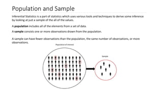
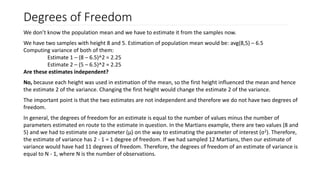
The document discusses inferential statistics, which involves drawing conclusions about a population from sample data, emphasizing the distinctions between populations and samples. It details various sampling methods, such as probability and non-probability sampling, and explains concepts like the sampling distribution and standard error. Additionally, it introduces the central limit theorem and discusses hypothesis testing and confidence intervals, as well as the significance of degrees of freedom in statistical estimates.