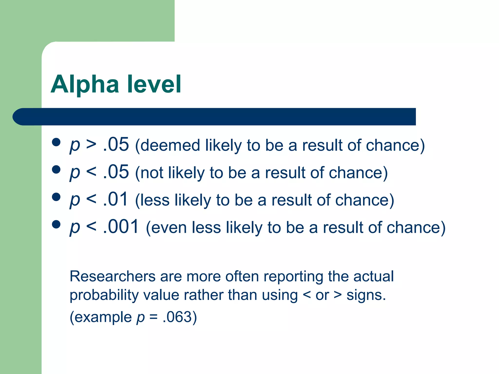
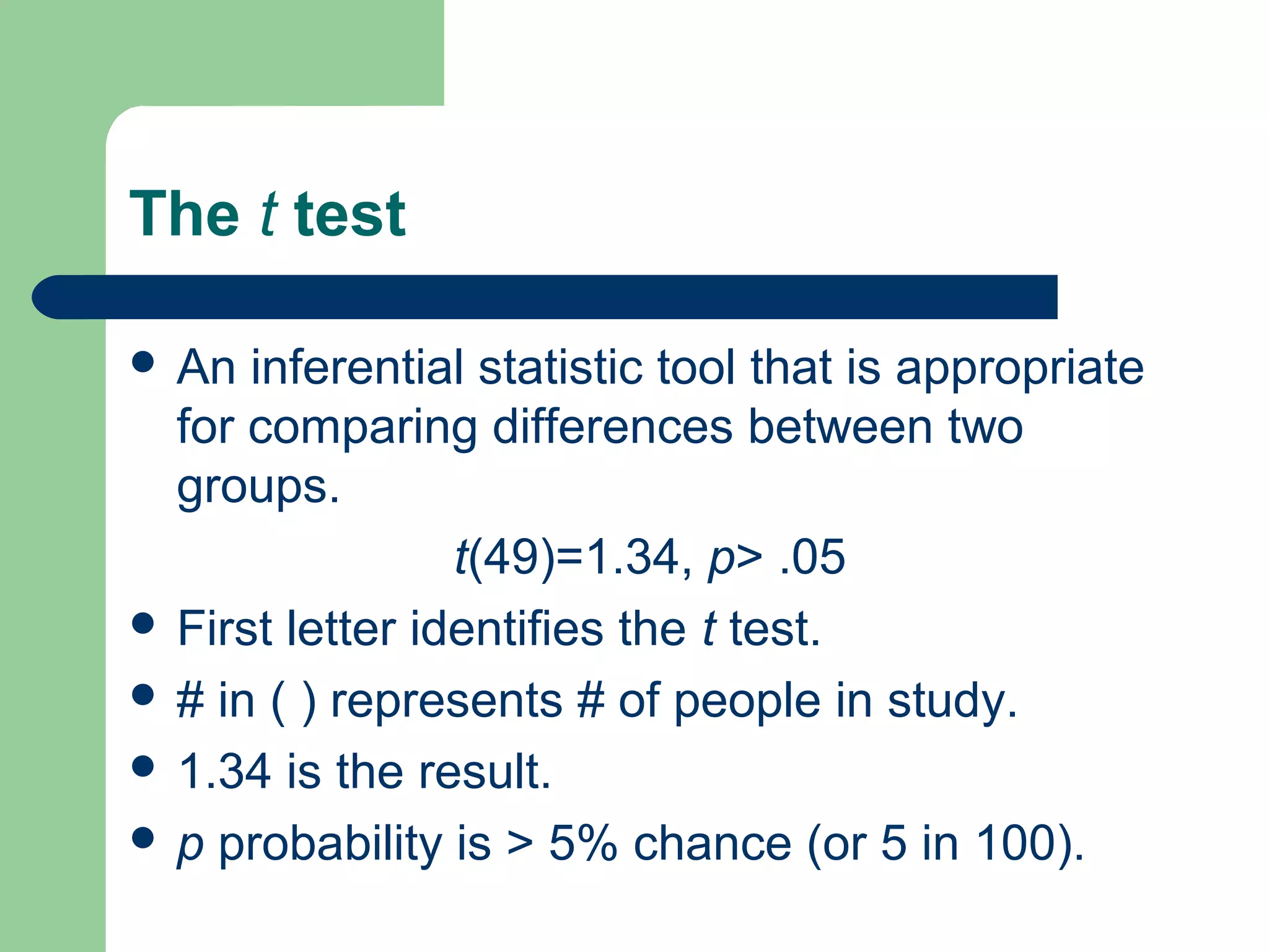
Inferential Statistics
Looking for the
possibility of a
chance occurrance
Erin White
EDPS 533
Key Question
 What is the probability that the difference
found between these samples would have
occurred if there were really no
differences in the total populations?
Alpha level
 p > .05 (deemed likely to be a result of chance)
 p < .05 (not likely to be a result of chance)
 p < .01 (less likely to be a result of chance)
 p < .001 (even less likely to be a result of chance)
Researchers are more often reporting the actual
probability value rather than using < or > signs.
(example p = .063)
The t test
 An inferential statistic tool that is appropriate
for comparing differences between two
groups.
t(49)=1.34, p> .05
 First letter identifies the t test.
 # in ( ) represents # of people in study.
 1.34 is the result.
 p probability is > 5% chance (or 5 in 100).
Analysis of Variance/ ANOVA
 Useful when comparing more than 2 groups (t test can only
compare 2 groups)
F(3,53)=26.26,p<.001
 F identifies the ANOVA
 3= # of mean scores compared + 1 (3+1=4 groups compared)
 53 = approx. # of people in study
 26.26= result of calculation of F ratio
 p< .001= probability is< 1 in 1,000 that the results are likely to
be a result of chance.
 The problem is that this doesn’t tell us exactly which group had
those differences. The researcher then may choose to make
paired comparisons. See figure 5.2 on p. 118
Analysis of Covariance/ ANCOVA
 This type of ANOVA is used when there is reason to believe
that the groups being compared were not the same before the
study began.
 Scores may be statistically adjusted to account for differences
on another variable.
 Example: Two groups of students are being compared, full and
part time. The full time students’ mean scores on a posttest
were 38; part time students’ mean was 34. They had been
given a pretest at the beginning of class in which they scored
full time-15 and part time-13. These groups were not
equivalent before the intervention, therefore pretest scores
were adjusted to come up with a more accurate probability
outcome.
Chi-Square (x²)
 A nonparametric tool- which means it can be used
without assumptions about the data distribution.(ex:
bell-shaped curve)
 This method is used when data is not in a form that
can be averaged.
x²(2, N = 120) = 12.39, p = .002
The probability of getting these results from a
sample if the population had no preference is 2 in
1,000.
Regression Analysis
 Researchers use this technique when there is
statistical significance (due to the correlation
coefficient) between variables to determine if one
can directly predict the other.
 They combine the correlation coefficients, means,
and standard deviations of each variable. They set it
up in equation form that will determine a direct
prediction.
Y = .35X + 2.50
(Y is the predicted # , X is a score of some sort)
Multiple Regression
 This is a more complex form of the regression analysis. It is
used when the relationship between more than two variables is
being studied.
Example: Y = .31X1 + 3.42X2 – 15.76
 Standard error of estimate- # calculated from the standard
deviation and correlation coefficient. As the correlation
between two variables goes up, the standard error of estimate
goes down- providing a better prediction.
 Confidence interval- these are used to increase the standard
error of estimate for greater confidence in their prediction.
 See figure 5.3 on p. 122
Statistical Significance
 When a difference between groups is labeled as unlikely to
have occurred by chance, it is labeled as statistically
significant. (p =<.05)
 Depends on size of the difference or relationship (correlation
coefficient), # of participants in the study.
 Remember, identifying a cause for the significance and taking
into consideration the effects of extraneous variables would be
practicing good research strategy.
 Effect size- A calculated standardized difference between
groups. Subtract the mean of one group from the mean of
another then divide by a standard deviation. Researchers
typically look for a large effect size. Cohen’s d is a current
technique that recommends that small, medium, and large
differences have corresponding values of .20, .50, & .80.
Null Hypothesis
 Often the form in which data will be analyzed in the
results section of a study.
 May be “rejected” or “failed to reject”.
 Rejecting occurs when the directional or
nondirectional hypotheses are correct.
 Failure to reject occurs when researchers allow for
the possibility that new data could reject the
hypothesis.
 ***one-tailed test-refers to a study that did not use a
null hypothesis.
Interpreting Graphs
 Be very critical of the visuals you find in a
research study.
 Graphs can be very misleading, whether
intentional or not.
 Pay attention to the #’s on the scale and not
just the visual impression.
 Read and re-read a graph, BE CRITICAL!!
Key Questions in Reviewing a Study
 Did the researchers clearly report what they
found?
 Did they report all of that information? If not,
did they explain why it was omitted?

Inferential Statistics

  • 1.
    Inferential Statistics Looking forthe possibility of a chance occurrance Erin White EDPS 533
  • 2.
    Key Question  Whatis the probability that the difference found between these samples would have occurred if there were really no differences in the total populations?
  • 3.
    Alpha level  p> .05 (deemed likely to be a result of chance)  p < .05 (not likely to be a result of chance)  p < .01 (less likely to be a result of chance)  p < .001 (even less likely to be a result of chance) Researchers are more often reporting the actual probability value rather than using < or > signs. (example p = .063)
  • 4.
    The t test An inferential statistic tool that is appropriate for comparing differences between two groups. t(49)=1.34, p> .05  First letter identifies the t test.  # in ( ) represents # of people in study.  1.34 is the result.  p probability is > 5% chance (or 5 in 100).
  • 5.
    Analysis of Variance/ANOVA  Useful when comparing more than 2 groups (t test can only compare 2 groups) F(3,53)=26.26,p<.001  F identifies the ANOVA  3= # of mean scores compared + 1 (3+1=4 groups compared)  53 = approx. # of people in study  26.26= result of calculation of F ratio  p< .001= probability is< 1 in 1,000 that the results are likely to be a result of chance.  The problem is that this doesn’t tell us exactly which group had those differences. The researcher then may choose to make paired comparisons. See figure 5.2 on p. 118
  • 6.
    Analysis of Covariance/ANCOVA  This type of ANOVA is used when there is reason to believe that the groups being compared were not the same before the study began.  Scores may be statistically adjusted to account for differences on another variable.  Example: Two groups of students are being compared, full and part time. The full time students’ mean scores on a posttest were 38; part time students’ mean was 34. They had been given a pretest at the beginning of class in which they scored full time-15 and part time-13. These groups were not equivalent before the intervention, therefore pretest scores were adjusted to come up with a more accurate probability outcome.
  • 7.
    Chi-Square (x²)  Anonparametric tool- which means it can be used without assumptions about the data distribution.(ex: bell-shaped curve)  This method is used when data is not in a form that can be averaged. x²(2, N = 120) = 12.39, p = .002 The probability of getting these results from a sample if the population had no preference is 2 in 1,000.
  • 8.
    Regression Analysis  Researchersuse this technique when there is statistical significance (due to the correlation coefficient) between variables to determine if one can directly predict the other.  They combine the correlation coefficients, means, and standard deviations of each variable. They set it up in equation form that will determine a direct prediction. Y = .35X + 2.50 (Y is the predicted # , X is a score of some sort)
  • 9.
    Multiple Regression  Thisis a more complex form of the regression analysis. It is used when the relationship between more than two variables is being studied. Example: Y = .31X1 + 3.42X2 – 15.76  Standard error of estimate- # calculated from the standard deviation and correlation coefficient. As the correlation between two variables goes up, the standard error of estimate goes down- providing a better prediction.  Confidence interval- these are used to increase the standard error of estimate for greater confidence in their prediction.  See figure 5.3 on p. 122
  • 10.
    Statistical Significance  Whena difference between groups is labeled as unlikely to have occurred by chance, it is labeled as statistically significant. (p =<.05)  Depends on size of the difference or relationship (correlation coefficient), # of participants in the study.  Remember, identifying a cause for the significance and taking into consideration the effects of extraneous variables would be practicing good research strategy.  Effect size- A calculated standardized difference between groups. Subtract the mean of one group from the mean of another then divide by a standard deviation. Researchers typically look for a large effect size. Cohen’s d is a current technique that recommends that small, medium, and large differences have corresponding values of .20, .50, & .80.
  • 11.
    Null Hypothesis  Oftenthe form in which data will be analyzed in the results section of a study.  May be “rejected” or “failed to reject”.  Rejecting occurs when the directional or nondirectional hypotheses are correct.  Failure to reject occurs when researchers allow for the possibility that new data could reject the hypothesis.  ***one-tailed test-refers to a study that did not use a null hypothesis.
  • 12.
    Interpreting Graphs  Bevery critical of the visuals you find in a research study.  Graphs can be very misleading, whether intentional or not.  Pay attention to the #’s on the scale and not just the visual impression.  Read and re-read a graph, BE CRITICAL!!
  • 13.
    Key Questions inReviewing a Study  Did the researchers clearly report what they found?  Did they report all of that information? If not, did they explain why it was omitted?