Hypothesis testing ppt

1. MACHINE LEARNING
21EL3202
Topic:
Hypothesis Testing
Department of CSE(H)
Session -
Dr. Nafees Akhter Farooqui
Assistant Professor
Department of CSE(H)

2. 2
AIM OF THE SESSION
To know students about the Hypothesis Testing and techniques.
INSTRUCTIONAL OBJECTIVES
This session is designed to:
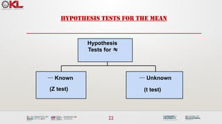
1. Basic Concepts of Hypothesis Testing.
2. Sampling Distribution.
3. Z Test
4. Genetic Algorithm
LEARNING OUTCOMES
At the end of this session, you should be able to:
1. Define Hypothesis Testing, Sampling Distribution and Genetic Algorithm
2. Implement the Hypothesis testing through the Z test.

3. 3
INTRODUCTION to Hypothesis Testing
 Hypothesis testing is a statistical method used to make decisions about a population based on a sample of data.
 A hypothesis test allows us to test the claim about the population and find out how likely it is to be true.
 The process of hypothesis testing involves testing two hypotheses: the null hypothesis and the alternative
hypothesis.
 The test statistic, and the critical value, P-value and the rejection region ( ), respectively are used for the
𝛼
Hypothesis testing.

4. 4
Types of Hypothesis
The process of hypothesis testing involves testing two hypothesis: the null hypothesis and the alternative
hypothesis.
• Null Hypothesis: The null hypothesis is a statement that assumes that there is no significant
difference between the sample data and the population data. The null hypothesis is usually denoted
as H0. The null hypothesis is assumed to be true unless the sample data provides sufficient evidence
to reject it.
• Alternative Hypothesis: The alternative hypothesis is a statement that assumes that there is a
significant difference between the sample data and the population data. The alternative hypothesis is
usually denoted as Ha or H1. The alternative hypothesis is assumed to be true if the sample data
provides sufficient evidence to reject the null hypothesis.

5. 5
The Hypothesis Testing Process
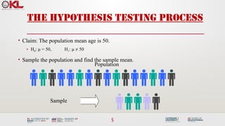
• Claim: The population mean age is 50.
• H0: μ = 50, H1: μ ≠ 50
• Sample the population and find the sample mean.
Population
Sample

6. 6
The Hypothesis Testing Process
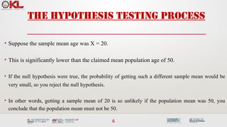
• Suppose the sample mean age was X = 20.
• This is significantly lower than the claimed mean population age of 50.
• If the null hypothesis were true, the probability of getting such a different sample mean would be
very small, so you reject the null hypothesis.
• In other words, getting a sample mean of 20 is so unlikely if the population mean was 50, you
conclude that the population mean must not be 50.

7. 7
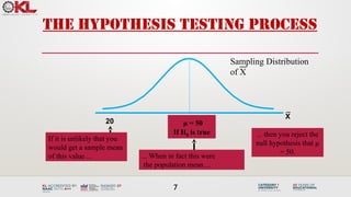
The Hypothesis Testing Process
μ = 50
If H0 is true
If it is unlikely that you
would get a sample mean
of this value ...
... then you reject the
null hypothesis that μ
= 50.
20
... When in fact this were
the population mean…
Sampling Distribution
of X
X

8. 8
THE TEST STATISTIC AND CRITICAL VALUES
 If the sample mean is close to the stated population mean, the null hypothesis is not rejected.
 If the sample mean is far from the stated population mean, the null hypothesis is rejected.
 How far is “far enough” to reject H0?
 The critical value of a test statistic creates a “line in the sand” for decision making -- it answers the
question of how far is far enough.

9. 9
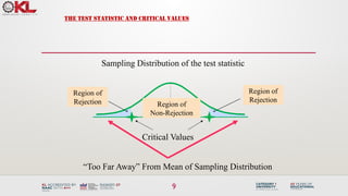
THE TEST STATISTIC AND CRITICAL VALUES
Critical Values
“Too Far Away” From Mean of Sampling Distribution
Sampling Distribution of the test statistic
Region of
Rejection
Region of
Rejection
Region of
Non-Rejection

10. 10
RISKS IN DECISION MAKING USING HYPOTHESIS TESTING
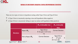
There are two types of errors in hypothesis testing called Type-I Error and Type-II Error
 A Type I Error is incorrectly rejecting a true null hypothesis (false negative).
 A Type II Error is incorrectly failing to reject an untrue null hypothesis (false positive).
𝑯𝟎 is Actually true 𝑯𝟎 is Actually
false
Decision
Reject 𝑯𝟎
Type-I Error
𝑃 ( )
𝑇𝑦𝑝𝑒 𝐼 𝐸𝑟𝑟𝑜𝑟
=α
Correct Decision
Fail to Reject 𝑯𝟎
Correct Decision Type-II Error
𝑃 ( II
𝑇𝑦𝑝𝑒
) =
𝐸𝑟𝑟𝑜𝑟 β

11. 11
RISKS IN DECISION MAKING USING HYPOTHESIS TESTING
Example for the Type-I Error:
For example, let’s assume that you make a claim that tomorrow the stock price will be the highest in the market. here the
alternate statements or hypotheses would be something like this,
H0 = The stock prices will not increase tomorrow
H1 = The stock prices will increase tomorrow
Now if we do hypothesis testing and the null hypothesis is proved to be correct, but due to lack of data and based on our
past experience, if we reject the null hypothesis, then there will be a Type-I error.

12. 12
RISKS IN DECISION MAKING USING HYPOTHESIS TESTING
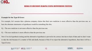
Example for the Type-II Error:
For example, let’s assume that a pharma company claims that their new medicine is more effective than the previous one. so
here the alternate statements or hypotheses would be something like this,
H0 = The new medicine is not more effective than the previous one
H1 = The new medicine is more effective than the previous one
Now if we do hypothesis testing and the alternative hypothesis is proved to be correct, but due to lack of data and we don’t want
to take the risk because it’s a matter of life and death, because of this if we reject the alternative hypothesis, then there will be a
Type-II error.

13. 13
• A sampling distribution refers to a probability distribution of a statistic that comes from choosing random samples
of a given population. Also known as a finite-sample distribution, it represents the distribution of frequencies on
how spread apart various outcomes will be for a specific population.
• The sampling distribution depends on multiple factors – the statistics, sample size, sampling process, and the
overall population. It is used to help calculate statistics such as means, ranges, variances, and standard deviations
for the given sample.
SAMPLING DISTRIBUTION

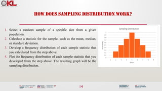
14. HOW DOES SAMPLING DISTRIBUTION WORK?
1. Select a random sample of a specific size from a given
population.
2. Calculate a statistic for the sample, such as the mean, median,
or standard deviation.
3. Develop a frequency distribution of each sample statistic that
you calculated from the step above.
4. Plot the frequency distribution of each sample statistic that you
developed from the step above. The resulting graph will be the
sampling distribution.
14

15. 15
For example, in South America, you randomly select data about the heights of 10-year-old children, and you
calculate the mean for 100 of the children. You also randomly select data from North America and calculate the
mean height for one hundred 10-year-old children.
As we continue to find the average heights for each sample group of children from each continent, we can calculate
the mean of the sampling distribution by finding the mean of all the average heights of each sample group. Not only
can it be computed for the mean, but it can also be calculated for other statistics such as standard deviation and
variance.
PRACTICAL EXAMPLE

16. 16
IMPORTANCE OF USING A SAMPLING DISTRIBUTION
 Most of the cases the population is in large size, it is important to use a sampling distribution so that you
can randomly select a subset of the entire population. It helps to eliminate variability when you are doing
research or gathering statistical data.
 It also helps make the data easier to manage and builds a foundation for statistical inferencing, which leads
to making inferences for the whole population.

17. 17
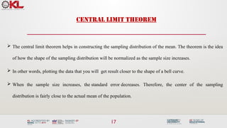
CENTRAL LIMIT THEOREM
 The central limit theorem helps in constructing the sampling distribution of the mean. The theorem is the idea
of how the shape of the sampling distribution will be normalized as the sample size increases.
 In other words, plotting the data that you will get result closer to the shape of a bell curve.
 When the sample size increases, the standard error decreases. Therefore, the center of the sampling
distribution is fairly close to the actual mean of the population.

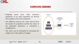
18. SAMPLING ERRORS
• Sampling errors occur when numerical
parameters of an entire population are derived
from samples of the entire population.
• The difference between the values derived from
the sample of a population and the true values of
the population parameters is considered a
sampling error.
• The errors can be eliminated by increasing the
sample size or the number of samples.
18

19. PRACTICAL EXAMPLE
19
 Suppose the producers of Company XYZ want to determine the viewership of a local program that airs twice a week. The
producers will need to determine the samples that can represent various types of viewers. They may need to consider factors
like age, level of education, and gender.
For example, people between the ages of 14 and 18 usually have fewer commitments, and most of them can spare time to
watch the program twice weekly. On the contrary, people between the age of 18 and 35 usually have tighter schedules and will
not have time to watch TV.
Hence, it is important to draw a sample proportionately. Otherwise, the results will not represent the real population.
Since the exact population parameter is not known, sampling errors for samples are generally unknown. However, analysts can
use analytical methods to measure the amount of variation caused by sampling errors.

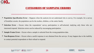
20. CATEGORIES OF SAMPLING ERRORS
20
 Population Specification Error – Happens when the analysts do not understand who to survey. For example, for a survey
of breakfast cereals, the population can be the mother, children, or the entire family.
 Selection Error – Occurs when the respondents’ survey participation is self-selected, implying only those who are
interested respond. Selection errors can be reduced by encouraging participation.
 Sample Frame Error – Occurs when a sample is selected from the wrong population data.
 Non-Response Error – Occurs when a useful response is not obtained from the surveys. It may happen due to the inability
to contact potential respondents or their refusal to respond.

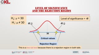
21. LEVEL OF SIGNIFICANCE
AND THE REJECTION REGION
Level of significance = a
This is a two-tail test because there is a rejection region in both tails
H0: μ = 30
H1: μ ≠ 30
Critical values
Rejection Region
/2
30
a
/2
a

22. 22
HYPOTHESIS TESTS FOR THE MEAN
 Known  Unknown
Hypothesis
Tests for 
(Z test) (t test)

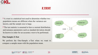
23. Z TEST
A z-test is a statistical test used to determine whether two
population means are different when the variances are
known, and the sample size is large.
The test statistic is assumed to have a normal distribution,
and nuisance parameters such as standard deviation should
be known in order for an accurate z-test to be performed.
One-Sample Z-Test
We perform the One-Sample z-Test when we want to
compare a sample mean with the population mean.
23

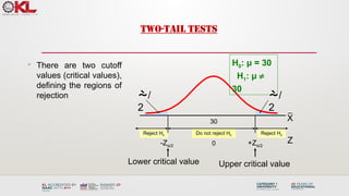
24. Do not reject H0 Reject H0
Reject H0
 There are two cutoff
values (critical values),
defining the regions of
rejection
TWO-TAIL TESTS
/
2
-Zα/2 0
H0: μ = 30
H1: μ ¹
30
+Zα/2
/
2
Lower critical value Upper critical value
30
Z
X

25. 25
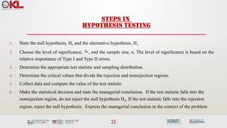
STEPS IN
HYPOTHESIS TESTING
1. State the null hypothesis, H0 and the alternative hypothesis, H1
2. Choose the level of significance, , and the sample size, n. The level of significance is based on the
relative importance of Type I and Type II errors.
3. Determine the appropriate test statistic and sampling distribution.
4. Determine the critical values that divide the rejection and nonrejection regions.
5. Collect data and compute the value of the test statistic
6. Make the statistical decision and state the managerial conclusion. If the test statistic falls into the
nonrejection region, do not reject the null hypothesis H0. If the test statistic falls into the rejection
region, reject the null hypothesis. Express the managerial conclusion in the context of the problem

26. 26
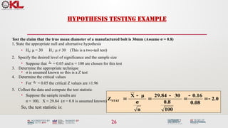
HYPOTHESIS TESTING EXAMPLE
Test the claim that the true mean diameter of a manufactured bolt is 30mm.(Assume σ = 0.8)
1. State the appropriate null and alternative hypothesis
• H0: μ = 30 H1: μ ≠ 30 (This is a two-tail test)
2. Specify the desired level of significance and the sample size
• Suppose that  = 0.05 and n = 100 are chosen for this test
3. Determine the appropriate technique
• σ is assumed known so this is a Z test
4. Determine the critical values
• For  = 0.05 the critical Z values are ±1.96
5. Collect the data and compute the test statistic
• Suppose the sample results are
n = 100, X = 29.84 (σ = 0.8 is assumed known)
So, the test statistic is:
2.0
0.08
.16
0
100
0.8
30
29.84
n
σ
μ
X
ZSTAT 








27. Reject H0 Do not reject H0
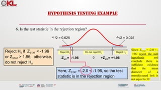
HYPOTHESIS TESTING EXAMPLE
6. Is the test statistic in the rejection region?
/2 = 0.025
-Zα/2 = -1.96 0
Reject H0 if ZSTAT < -1.96
or ZSTAT > 1.96; otherwise,
do not reject H0
/2 = 0.025
Reject H0
+Zα/2 = +1.96
Here, ZSTAT = -2.0 < -1.96, so the test
statistic is in the rejection region
Since ZSTAT = -2.0 < -
1.96, reject the null
hypothesis and
conclude there is
sufficient evidence
that the mean
diameter of a
manufactured bolt is
not equal to 30

28. 28
P-VALUE APPROACH TO TESTING
p-value: Probability of obtaining a test statistic equal to or more extreme
than the observed sample value given H0 is true
The p-value is also called the observed level of significance
It is the smallest value of  for which H0 can be rejected

29. 29
P-VALUE APPROACH TO TESTING:INTERPRETING THE P-
VALUE
• Compare the p-value with 
• If p-value <  , reject H0
• If p-value   , do not reject H0
• Remember
• If the p-value is low then H0 must go

30. 30
5 STEPS FOR P-VALUE APPROACH TO
HYPOTHESIS TESTING
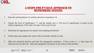
1. State the null hypothesis, H0 and the alternative hypothesis, H1
2. Choose the level of significance, , and the sample size, n. The level of significance is based on the
relative importance of the risks of a type I and a type II error.
3. Determine the appropriate test statistic and sampling distribution
4. Collect data and compute the value of the test statistic and the p-value
5. Make the statistical decision and state the managerial conclusion. If the p-value is < α then reject H0,
otherwise do not reject H0. State the managerial conclusion in the context of the problem

31. 31
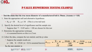
P-VALUE HYPOTHESIS TESTING EXAMPLE
• Test the claim that the true mean diameter of a manufactured bolt is 30mm. (Assume σ = 0.8)
1. State the appropriate null and alternative hypotheses
• H0: μ = 30 H1: μ ≠ 30 (This is a two-tail test)
2. Specify the desired level of significance and the sample size
• Suppose that  = 0.05 and n = 100 are chosen for this test
3. Determine the appropriate technique
• σ is assumed known so this is a Z test.
4. Collect the data, compute the test statistic and the p-value
• Suppose the sample results are
n = 100, X = 29.84 (σ = 0.8 is assumed known)
So, the test statistic is:
2.0
0.08
.16
0
100
0.8
30
29.84
n
σ
μ
X
ZSTAT 








32. P-VALUE HYPOTHESIS TESTING EXAMPLE:
CALCULATING THE P-VALUE
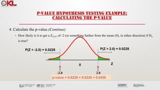
4. Calculate the p-value.(Continue)
• How likely is it to get a ZSTAT of -2 (or something further from the mean (0), in either direction) if H0
is true?
p-value = 0.0228 + 0.0228 = 0.0456
P(Z < -2.0) = 0.0228
0
-2.0
Z
2.0
P(Z > 2.0) = 0.0228

33. 33
P-VALUE HYPOTHESIS TESTING EXAMPLE:CALCULATING
THE P-VALUE
5. Is the p-value < α?
• Since p-value = 0.0456 < α = 0.05 Reject H0
State the managerial conclusion in the context of the situation.
• There is sufficient evidence to conclude the mean diameter of a manufactured bolt is
not equal to 30mm

34. 34
CONNECTION BETWEEN TWO TAIL TESTS AND
CONFIDENCE INTERVALS
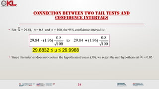
• For X = 29.84, σ = 0.8 and n = 100, the 95% confidence interval is:
29.6832 ≤ μ ≤ 29.9968
• Since this interval does not contain the hypothesized mean (30), we reject the null hypothesis at  = 0.05
100
0.8
(1.96)
29.84
to
100
0.8
(1.96)
-
29.84 

35. 35
THANK YOU