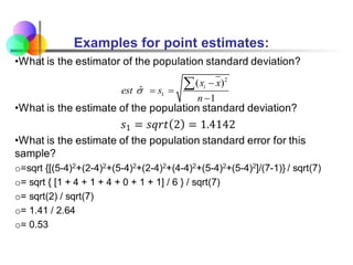
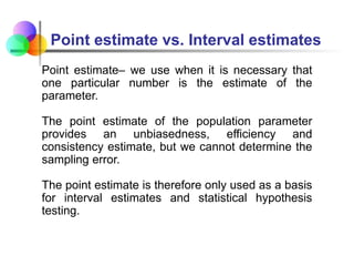
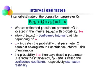
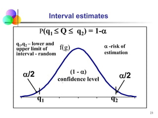
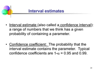
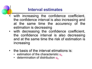
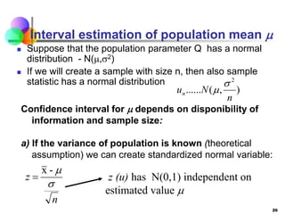
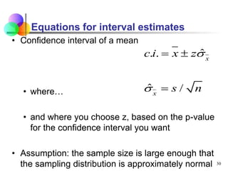
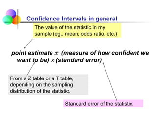
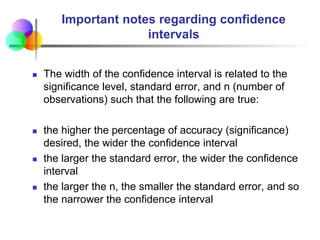
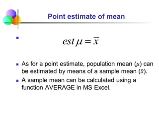
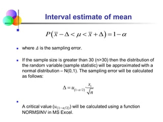
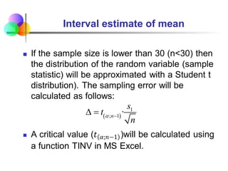
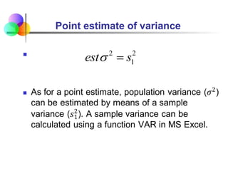
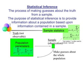
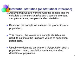
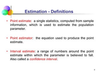
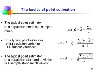
Statistical inference involves using sample statistics to make estimates about unknown population parameters. Point estimates provide a single value, such as using the sample mean (x̅) to estimate the population mean (μ). Interval estimates provide a range of values that the population parameter is likely to fall within, such as a 95% confidence interval. The width of the confidence interval depends on factors like the desired confidence level, sample size, and standard error - generally, larger sample sizes and lower standard errors result in narrower intervals.

1. Statistical inference: point and
interval estimate

2. Statistical Inference
The process of making guesses about the truth
from a sample.
The purpose of statistical inference is to provide
information about a population based upon
information contained in a sample.
Sample
(observation)
Make guesses about
the whole
population
Truth (not
observable)
N
x
N
i
i
2
1
2
)
( 





N
x
N
i


 1

Population
parameters
1
)
(
ˆ
2
1
2
2






n
X
x
s
n
n
i
i

n
x
X
n
i
n



 1
̂
Sample statistics
*hat notation ^ is often used to
indicate “estimate”

3. Statistical inference
 The reasons to make guesses about the whole
population based on sample statistics:
 Contacting the entire population is too time consuming.
 The cost of studying all the items in the population is often
too expensive.
 The sample results are usually adequate.
 The destructive nature of certain tests.
 The physical impossibility of checking all items.
As we mentioned before, there are several methods of
sampling (simple random sample is the most widely used
method, others are: systematic sampling, stratified sampling,
and cluster sampling).

4. 4
Inferential statistics (or Statistical inference)
 Assume that we are working with the sample and we
calculate a sample statistics such: sample average,
sample variance, sample standard deviation.
 Based on the sample we assume the properties of a
population.
 This means , the values of a sample statistics are
used to estimate the unknown values of population
parameters.
 Usually we estimate parameters of population such :
population mean, population variance, standard
deviation of population.

5. Statistics vs. Parameters
 A population – is the collection of all elements of interest.
 Population parameter – the true value/true effect in the
entire population of interest.
 E.g., the true mean vitamin D level in all middle-aged and older
European men is 62 nmol/L.
 A sample – is a subset of a population.
 Sample Statistic – any summary measure calculated from
data; e.g., could be a mean.
 E.g., the mean vitamin D level in a sample of 100 men is 63 nmol/L.

6. Symbols:
PARAMETERS OF
POPULATION
SAMPLE STATISTICS
N – size of population n - sample size
 - population mean
s – sample standard
deviation
Q – population in general

7. 7
Graphicaly
Sample
with size n
Symbols:
parameters of population:
, 2, , N
Generally: Q
sample characteristics :
Generally:un
n
s
x ,
,
s
, 2
Population – size N,
resp.  (infinity)

8. What we have accomplished with sampling
distributions
• Given a population parameter, we know that a
sample statistic will produce a better estimate of the
population parameter when the sample is larger
(better means more accurate and normally
distributed).
8

9. Estimation - Definitions
• Point estimate: a single statistics, computed from sample
information, which is used to estimate the population
parameter.
• Point estimator: the equation used to produce the point
estimate.
• Interval estimate: a range of numbers around the point
estimate within which the parameter is believed to fall.
Also called a confidence interval.
9

10. Mathematical Theory…
The Central Limit Theorem!
If all possible random samples, each of size n, are taken from
any population with a mean  and a standard deviation , the
sampling distribution of the sample means (averages) will:

 
x
1. have mean:
n
x

 
2. have standard deviation:
3. be approximately normally distributed regardless of the shape
of the parent population (normality improves with larger n).

11. Symbol Check
x
 The mean of the sample means.
x
 The standard deviation of the sample means.
Also called “the standard error of the mean.”

12. The Central Limit Theorem


13. The Central Limit Theorem


14. The basics of point estimation
• The typical point estimator
of a population mean is a sample
mean:
• The typical point estimator
of a population variance
is a sample variance:
• The typical point estimator
of a population standard deviation
is a sample standard deviation:
ˆ i
x
est x
n


 
14
2
2 2
1
( )
ˆ
1
i
x x
est s
n


 


2
1
( )
ˆ
1
i
x x
est s
n


 



15. Typical point estimator for standard errors
• Estimated standard error
of samples drawn from a
population:
15
ˆ
ˆx
s
n n

  

16. Choosing a good estimator
You can technically use any equation you want as a point estimator, but the
most popular ones have certain desirable properties.
•Unbiasedness: The sampling distribution for the estimator
‘centers’ around the parameter (on average, the estimator
gives the correct value for the parameter).
•Efficiency: If at the same sample size one unbiased estimator
has a smaller sampling error than another unbiased estimator,
the first one is more efficient.
•Consistency: The value of the estimator gets closer to the
parameter as sample size increases. Consistent estimators
may be biased, but the bias must become smaller as the
sample size increases if the consistency property holds true.
16

17. Examples for point estimates:
Given the following sample of seven observations:
5, 2, 5, 2, 4, 5, 5
• What is the estimator of the population mean?
• What is the estimate of the population mean?
• What is the estimator of the population variance?
• What is the estimate of the population variance?
• What is the estimator of the population standard deviation?
• What is the estimate of the population standard deviation?
• What is the estimate of the population standard error for
this sample?
17

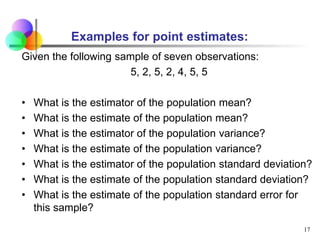
18. Examples for point estimates:
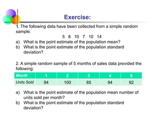
Given the following sample of seven observations:
5, 2, 5, 2, 4, 5, 5
 What is the estimator of the population mean?
 What is the estimate of the population mean?
(5+2+5+2+4+5+5) / 7 = 28 / 7 = 4
 What is the estimator of the population variance?
 What is the estimate of the population variance?
[(5-4)2+(2-4)2+(5-4)2+(2-4)2+(4-4)2+(5-4)2+(5-4)2]/6=2
18
ˆ i
x
est x
n


 
2
2 2
1
( )
ˆ
1
i
x x
est s
n


 



19. Examples for point estimates:
2
1
( )
ˆ
1
i
x x
est s
n


 



20. Exercise:
1. The following data have been collected from a simple random
sample.
5 8 10 7 10 14
a) What is the point estimate of the population mean?
b) What is the point estimate of the population standard
deviation?
2. A simple random sample of 5 months of sales data provided the
following:
a) What is the point estimate of the population mean number of
units sold per month?
b) What is the point estimate of the population standard
deviation?
Month 1 2 3 4 5
Units Sold 94 100 85 94 92

21. Point estimate– we use when it is necessary that
one particular number is the estimate of the
parameter.
The point estimate of the population parameter
provides an unbiasedness, efficiency and
consistency estimate, but we cannot determine the
sampling error.
The point estimate is therefore only used as a basis
for interval estimates and statistical hypothesis
testing.
Point estimate vs. Interval estimates

22. Interval estimates
Interval estimate of the population parameter Q:
• Where: estimated population parameter Q is
located in the interval (q1,q2) with probability 1-a
• interval (q1,q2) = confidence interval and it is
depending on a
• a  indicates the probability that parameter Q
does not belong into the confidence interval - risk
of estimation
• the probability 1-a then says that the parameter
Q is from the interval (q1, q2) and is called the
confidence coefficient, respectively estimation
reliability
a



 1
)
q
Q
q
(
P 2
1

23. 23
Interval estimates
q1 q2
(1 - a)
confidence level
a/2 a/2
P(q1  Q  q2) = 1-a
a -risk of
estimation
q1,q2 – lower and
upper limit of
interval - random
f(g)

24. • Interval estimate (also called a confidence interval):
a range of numbers that we think has a given
probability of containing a parameter.
• Confidence coefficient: The probability that the
interval estimate contains the parameter. Typical
confidence coefficients are 1-a = 0.95 and 0.99.
24
Interval estimates

25. • with increasing the confidence coefficient,
the confidence interval is also increasing and
at the same time the accurency of the
estimation is decreasing
• with decreasing the confidence coefficient,
the confidence interval is also decreasing
and at the same time the risk of estimation is
increasing
• the basis of the interval etimations is:
• estimation of the characteristic un
• determination of distribution un
Interval estimates

26. 26
Interval estimation of population mean 
 Suppose that the population parameter Q has a normal
distribution - N(,2)
 If we will create a sample with size n, then also sample
statistic has a normal distribution
)
,
(
......
2
n
N
un


n
z


-
x
 z (u) has N(0,1) independent on
estimated value 
Confidence interval for  depends on disponibility of
information and sample size:
a) If the variance of population is known (theoretical
assumption) we can create standardized normal variable:

27. 27
1 1
2 2
1-
x - μ
P z z
σ
n
a a a
 
 
 
   
 
 
 
 
1
2
z a

 1
2
z a

1 - a
f(u)
according to N (0,1) we
determine q1, q2 = z1-a/2
Interval estimation of population mean 

28. 28
1 1
2 2
x 1-
n n
P x z z
a a
 
 a
 
 
    
 
 
After transformation we get following equation:
 - sampling error
 - half of the interval,
determinates accurancy of the
estimation,
Interval estimate is actually point
estimate  , e.g. Δ
x 
Δ
x 
Δ
x 
Interval estimation of population mean 

29. 29
b) The population variance is unknown
est 2 = s1
2 , and the sample size is large, n > 30
1
1
2 n
s
x z a


c) If the population variance is unknown
est 2 = s1
2 , and the sample size is small
(less than 30), n  30
n
s
t
x 1
1)
-
(n
a

ta(n-1) –critical value of
Student’s distribution at
alfa level and at degrees
of freedom
We can use N(0,1)
Interval estimation of population mean 

30. Equations for interval estimates
• Confidence interval of a mean
• where…
• and where you choose z, based on the p-value
for the confidence interval you want
• Assumption: the sample size is large enough that
the sampling distribution is approximately normal
ˆ
. . x
c i x z
 
ˆ /
x
s n
 
30

31. Notes on interval estimates
• Usually, we are not given z. Instead we start with a
desired confidence interval (e.g., 95% confidence),
and we select an appropriate z – score.
• We generally use a 2-tailed distribution in which ½ of
the confidence interval is on each side of the sample
mean.
31

32. Equations for interval estimates
• Example: find c.i. when Ybar =10.2, s=10.1, N=1055, interval=95%.
• z is derived from the 95% value: what value of z leaves 95% in the
middle and 2.5 % on each end of a distribution?
• For p = .975, z = 1.96
• The standard error is s/SQRT(n) = 10.1/SQRT(1055) = .31095
• Top of the confidence interval is 10.2 + 1.96*.31095 = 10.8095
• The bottom of the interval is 10.2 – 1.96*.31095 = 9.5905
• Hence, the confidence interval is 9.59 to 10.81
32

33. Confidence Intervals in general
point estimate  (measure of how confident we
want to be)  (standard error)
The value of the statistic in my
sample (eg., mean, odds ratio, etc.)
From a Z table or a T table,
depending on the sampling
distribution of the statistic.
Standard error of the statistic.

34. Common “Z” levels of confidence
 Confidence levels and corresponding Z values:
 Commonly used confidence levels are 95%
and 99%
Confidence
Level
Z value
1.28
1.645
1.96
2.33
2.58
3.08
3.27
80%
90%
95%
98%
99%
99.8%
99.9%

35. Confidence Interval for the Variance and
Standard Deviation of a Normal Distribution

36. Summary

37. Important notes regarding confidence
intervals
 The width of the confidence interval is related to the
significance level, standard error, and n (number of
observations) such that the following are true:
 the higher the percentage of accuracy (significance)
desired, the wider the confidence interval
 the larger the standard error, the wider the confidence
interval
 the larger the n, the smaller the standard error, and so
the narrower the confidence interval

38. Important note regarding the sample size
and sampling error
 The lower the desired sampling error the larger the
sample size must be.
 Note: Sampling error is influenced by:
 confidence level - we can influence the confidence level
 (sample) standard deviation - we can't influence the
variability within the sample
 sample size - we can influence the sample size

39. Point estimate of mean

est x
 

40. Interval estimate of mean

 
1
1 /2
·
s
u
n
a

 
  1
P x x
 a
       

41. Interval estimate of mean

 
1
; 1
·
n
s
t
n
a 
 

42. Point estimate of variance
 2 2
1
est s
 

43. Interval estimate of variance
 
 
 
 
2 2
1 1
2
2 2
/2; 1 1 /2; 1
1 · 1 ·
1
n n
n s n s
P
a a
 a
 
  
 
 
 
   
 
 

44. Point estimate of standard deviation

1
est s
 

45. Interval estimate of standard deviation
  
 
 
 
2 2
1 1
2
2 2
/2; 1 1 /2; 1
1 · 1 ·
1
n n
n s n s
P
a a
 a
 
  
 
 
 
   
 
 

46. Calculating the sample size

 
2
2 1
1 /2 2
·
s
n u a




47. Next topic
 Hypothesis testing
Thank you!
Have a nice day!