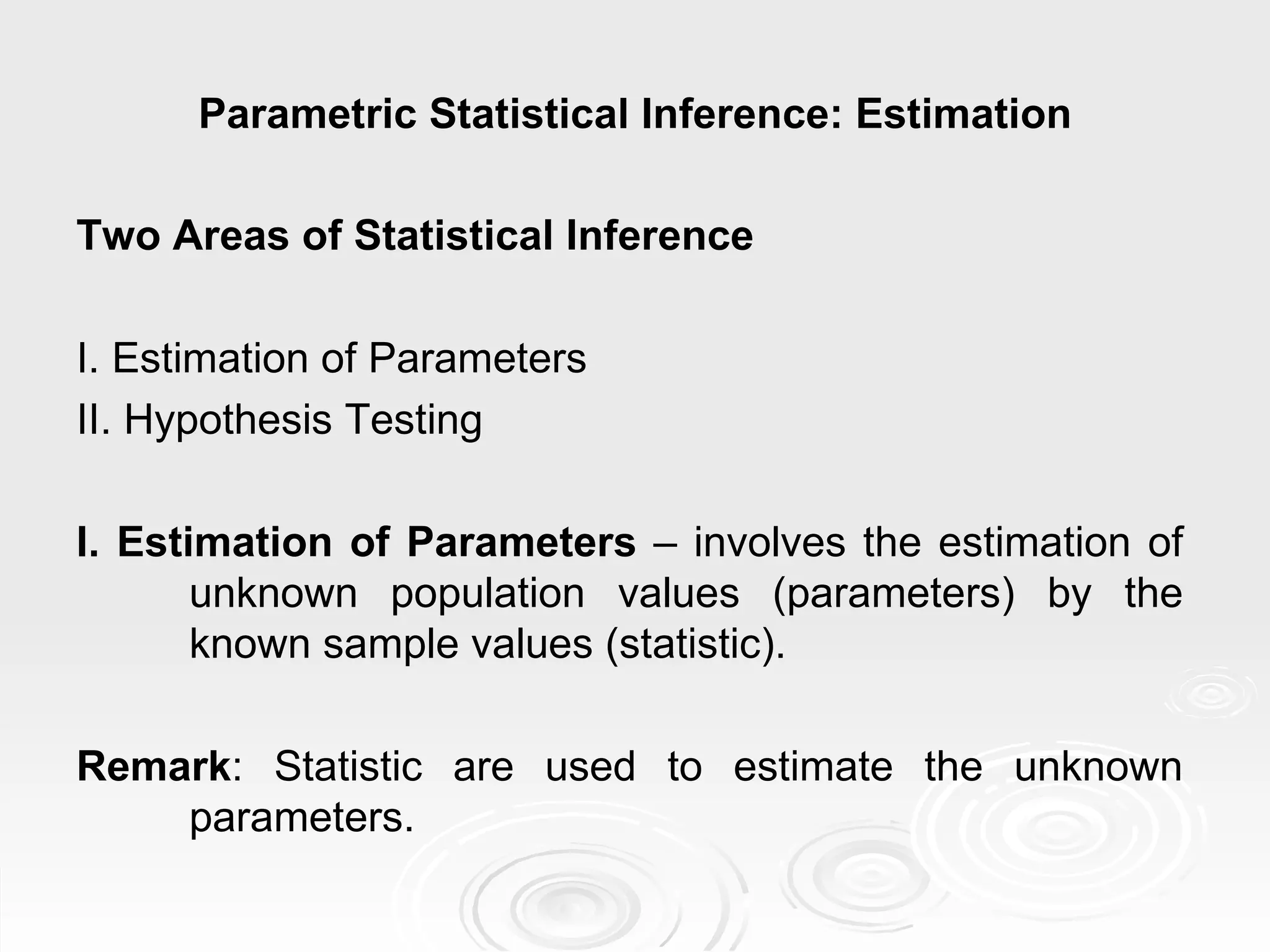
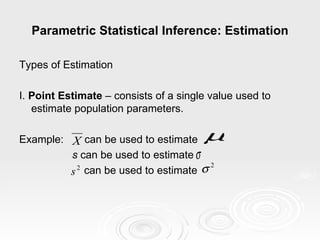
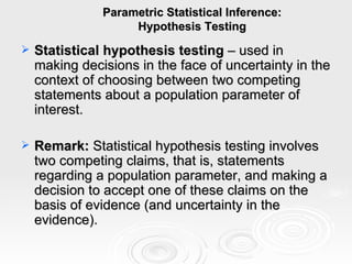
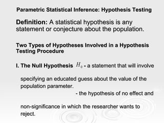
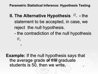
This document discusses two main areas of statistical inference: estimation and hypothesis testing. It provides details on point estimation and confidence interval estimation when estimating population parameters. It also explains the key concepts involved in hypothesis testing such as the null and alternative hypotheses, types of errors, critical regions, test statistics, and p-values. Examples are provided to illustrate estimating population means and proportions as well as conducting hypothesis tests.

1. Parametric Statistical Inference: Estimation Two Areas of Statistical Inference I. Estimation of Parameters II. Hypothesis Testing I. Estimation of Parameters – involves the estimation of unknown population values (parameters) by the known sample values (statistic). Remark : Statistic are used to estimate the unknown parameters.

2. Parametric Statistical Inference: Estimation Types of Estimation I. Point Estimate – consists of a single value used to estimate population parameters. Example: can be used to estimate s can be used to estimate can be used to estimate

3. Parametric Statistical Inference: Estimation II. A confidence – Interval Estimate – consists of an interval of numbers obtained from a point estimate, together with a percentage specifying how confident we are that the parameters lies in the interval. Example: Consider the following statement. A 95% confidence interval for the mean grade of graduate students is (1.0, 1.5). Remark: The number 95% or 0.95 is called the confidence coefficient or the degree of confidence. The end points (1.0, 1.5) that is 1.50 and 1.0 are respectively called the lower and upper confidence limits.

4. Parametric Statistical Inference: Estimation Remark: In general, we can always construct a 100% confidence interval. The Greek letter is referred as the level of significance and a fraction is called the confidence coefficient which is interpreted as the probability that the interval encloses the true value of the parameter. The following table presents the most commonly used confidence coefficients and the corresponding z – values. Confidence Coefficient 90% 0.10 1.282 .05 1.645 95% 0.05 1.645 0.025 1.960 99% 0.01 2.326 0.005 2.576

5. Estimating the Population Mean I. The Point Estimator of is . II. The Interval Estimator of is the confidence interval given by: 1. when is known. 2. when is unknown, where is the t-value with degrees of freedom.

6. Estimating the Population Mean Remark: If is unknown but for as long as , we still use (1) instead of (2). This explains the notion that the t is used only for small sample cases .

7. The Nature of t -Distribution develop by William Sealy Gosset (1896 – 1937), an employee of the Guinness Brewery in Dublin, where he interpreted data and planned barley experiments. his findings was under the pseudonym “student” because of the Guinness Company’s restrictive policy on publication by its employees.

8. The Nature of t -Distribution The Sampling Distribution William Sealy Gosset studied are then called Student’s t -distributions which is given by .

9. The Nature of t -Distribution Properties of the t -distribution 1. unimodal; 2. asymptotic to the horizontal axis; 3. symmetrical about zero; 4. dependent on v , the degrees of freedom (for the statistic under discussion, ). 5. more variable than the standard normal distribution, for ; 6. approximately standard normal if v is large. Definition: Degrees of freedom – the number of values that are free to vary after a sample statistic has been computed, and they tell the researcher which specific curve to use when a distribution consists of a family of curves.

10. Estimating the Population Mean Example 1: From a random sample of 16 applicants for certain graduate fellowships, the following statistics are obtained about their GRE scores , , a. Give the best point estimate of the population mean. b. Estimate the standard error of this estimate. c. Find a 95% confidence interval on this population mean.

11. Estimating the Population Mean Note: Example2: A study found that the average time it took a person to find a new job was 5.9 months. If a sample of 36 job seekers was surveyed, find the 99% confidence interval of the true population mean. Assume that the standard deviation is 0.8 month.

12. Estimating the Population Mean Doing with Excel: The expression in the confidence interval for the population mean can be obtained in excel software by entering = CONFIDENCE = - CONFIDENCE = + CONFIDENCE

13. Estimating the Population Proportion In a binomial experiment, the point estimator of the population proportion p is where x represents the number of successes in n trials. On the other hand, a confidence interval for population proportion p is given by: where and .

14. Estimating the Population Proportion Example 1: In a certain state, a survey of 500 workers showed that 45% belong to a union. Find the 90% confidence interval of the true proportion of workers who belong to a union.

15. Estimating the Population Proportion Example 2: A survey of 120 female freshmen showed that 18 did not wish to work after marriage. Find the 95% confidence interval of the true proportion of females who do not work after marriage.

16. Parametric Statistical Inference: Hypothesis Testing Statistical hypothesis testing – used in making decisions in the face of uncertainty in the context of choosing between two competing statements about a population parameter of interest. Remark: Statistical hypothesis testing involves two competing claims, that is, statements regarding a population parameter, and making a decision to accept one of these claims on the basis of evidence (and uncertainty in the evidence).

17. Parametric Statistical Inference: Hypothesis Testing Definition: A statistical hypothesis is any statement or conjecture about the population. Two Types of Hypotheses Involved in a Hypothesis Testing Procedure I. The Null Hypothesis - a statement that will involve specifying an educated guess about the value of the population parameter. - the hypothesis of no effect and non-significance in which the researcher wants to reject.

18. Parametric Statistical Inference: Hypothesis Testing II. The Alternative Hypothesis - the statement to be accepted, in case, we reject the null hypothesis. - the contradiction of the null hypothesis . Example: If the null hypothesis says that the average grade of the graduate students is 50, then we write, .

19. Parametric Statistical Inference: Hypothesis Testing Example: There are three possible alternative hypothesis which may be formulated from the preceding null hypothesis . a. (the average grade of the graduate students is less than 50) b. (the average grade of the graduate students is greater than 50) c. (the average grade of the graduate students is not equal to 50)

20. Parametric Statistical Inference: Hypothesis Testing Remarks: 1. The first two alternative hypotheses are called one-tailed or a directional test. 2. The third alternative hypothesis is called two-tailed or a non-directional test. Decision Rule – a criterion that specifies whether or not the null hypothesis should be rejected in favor of the alternative hypothesis.

21. Parametric Statistical Inference: Hypothesis Testing Remark: The decision is based on the value of a test statistic, the value of which is determined from sample measurements. Critical Region – the area under sampling distribution that includes unlikely sample outcomes which is also known as the rejection region. -the area where the null hypothesis is rejected.

22. Parametric Statistical Inference: Hypothesis Testing Acceptance Region –the region where the null hypothesis is accepted. Critical Value – the value between the critical region and the acceptance region

23. Parametric Statistical Inference: Hypothesis Testing Two Types of Errors that may be committed in rejecting or accepting the null hypothesis I. Type I Error – occurs when we reject the null hypothesis when it is true. - denoted by . II. Type II Error – occurs when we accept the null hypothesis when it is false. - denoted by .

24. Parametric Statistical Inference: Hypothesis Testing The following table displays the possible consequences in the decision to accept or reject the null hypothesis. Decision Null Hypothesis True False Reject Type I Correct Decision Accept Correct Type I Decision

25. Parametric Statistical Inference: Hypothesis Testing Remark: is called the level of significance which is interpreted as the maximum probability that the researcher is willing to commit a Type I Error. Remark: The acceptance of the null hypothesis does not mean that it is true but it is a result of insufficient evidence to reject it.

26. Parametric Statistical Inference: Hypothesis Testing Remark: and errors are related. For a fixed sample size n , an increase of results to a decrease in and a decrease in results to an increase in . However, decreasing the two errors simultaneously can only be achieved by increasing the sample size n . As increases, the size of the critical region also increases. Thus, if is rejected at , then will also be rejected at a level of significance higher than .

27. Parametric Statistical Inference: Hypothesis Testing In hypothesis testing procedure, the following steps are suggested: 1. State the null hypothesis and the alternative hypothesis. 2. Decide on the level of significance. 3. Determine the decision rule, the appropriate test statistic and the critical region. 4. Gather the given data and compute the value of the test statistic. Check the computed value if it falls inside the critical region or in the acceptance region. 5. Make the decision and state the conclusion in words.

28. Parametric Statistical Inference: Hypothesis Testing Remark: Alternatively, the p -value can also be used to make decision about the population of interest. Definition: The p -value represents the chance of generating a value as extreme as the observed value of the test statistic or something more extreme if the null hypothesis were true. Remark: The p-value serves to measure how much evidence we have against the null hypothesis. The smaller the p-value, the more evidence we have. Remark: If the p-value is less than the level of significance, then the null hypothesis is rejected, otherwise, the null hypothesis is accepted.