This document defines biometry and summarizes statistical methods for estimating population parameters from sample data. It begins by defining biometry as the application of statistical methods to biological problems, involving the measurement of life. It then discusses two types of estimation: point estimation, which provides a single value as an estimate, and interval estimation, which provides a range of values that the parameter is expected to fall within at a given confidence level. The document provides formulas and examples for constructing confidence intervals to estimate a single mean, the difference between two population means, and other parameters, depending on whether the population standard deviation is known or estimated from sample data, and whether sample sizes are large or small.

1. BIOMETRY

2. 1. Introduction
Definition of Statistics
Statistics is defined as study of numerical data based on
variation in nature.
• It is a science, which deals with collection, classification,
tabulation, summarization and analysis of quantitative data
or numerical facts.
• Statistics also refers to numerical and quantitative data
such as statistics of births, deaths, marriage, production,
yield, etc.

3. Applications of Statistics
• Currently, statistics is used as an analytical tool in
many fields of research.
• It has wide applications in almost all fields of study
– social science,agriculture, medicine, engineering, etc.
– it provides scientific methods for appropriate data
collection, analysis and summarization of data, and
inferential statistical methods for drawing conclusions
in the face of uncertainty.

4. Applications of Statistics
• The application of statistical methods to the
solution of biological problems is known as
biometry, biological statistics or bio-statistics.
• The word biometry comes from two Greek roots:
'bios' mean life and metron mean 'to measure'.
• Thus, biometry literally means the measurement
of life.

5. The Agricultural Roots of Experimental Design
• Statistical methods for designing and analyzing experiments
appeared first in agricultural research.
• Today, most statisticians credit Sir Ronald A. Fisher with the
original development of the theory and practice of statistically
designed experiments.
• Fisher worked at the Rothamsted Experimental Station in
England from 1919 until 1933.
• During that time, Fisher carefully studied results of wheat
experiments conducted at Rothamsted using data going back to
experiments conducted in 1843.
• In his investigations, he discovered that many false or ambiguous
claims from these early experiments stemmed from four major
shortcomings.

6. These four major shortcomings were:
1. Treatments, such as the variety of wheat being tested, were not
randomly assigned to experimental unit, e.g. growing areas
within a farm.
2. Agronomists were aware of some major causes of variation,
such as soil condition and rainfall, but they did not know how to
balance assignment of treatments to experimental material to
remove the effects of these known sources of variation.
3. Agronomists either designed experiments using too many
replicates or not enough.
4. Once the data were collected, agronomists interpreted the results
without taking into account the variability of their
measurements.

7. • In reality, average yields of wheat were contaminated by
uncontrolled sources of variation, such as soil conditions
and rainfall.
• In Fisher’s day, two agronomists might have completely
different interpretations of differences between wheat
varieties.
– One might claim that one variety yielded higher than the others
(i.e., he assumes true genotypic differences).
– Another agronomist viewing the same data might argue that
variety differences were just random measurement variation
rather than repeatable differences between the wheat varieties
(i.e., the observed differences were simply due to error).

8. What Did Fisher Do? (His Basic Contributions)
After understanding the problems, Fisher developed techniques for
settling these issues.
• His methods fall into two general categories:
1. Methods for designing experiments, and
2. Methods for analyzing and interpreting data from statistically
designed experiments.
His methods were published in a series of three books:
1. Statistical Principles for Research Workers (Fisher, 1925),
2. The Arrangement of Field Experiments (Fisher, 1926),
3. The Design of Experiments (Fisher, 1935).
• His last book was used for many years as the basic text for modern
statistical methods, and most of today’s introductory statistical
textbooks still use much of the terminology, concepts and
conventions set by Sir Fisher in 1935.

9. Divisions of Statistics
1. Descriptive Statistics: Are methods, which are
used to describe a set of data using the
measures of central tendency (mean, median,
mode) and measures of dispersion (standard
deviation, variance) without involving
generalization.
 Helps in summarizing and organizing data so as to
make them readable for users, e.g. mean, median,
mode, standard deviation, etc.

10. Divisions of Statistics
2. Inferential Statistics: It is a statistics, which
helps in drawing conclusions about the whole
population based on data from some of its parts
(samples).
• We often make decisions about the whole
population on the basis of sample information
using probability theory.

11. Inferential Statistics
Reading Assignment:
– Probability Distributions (Binomial, Poisson, Normal
(Gaussian)),
– Sampling Methods (probability (simple random
sampling, systematic sampling, stratified sampling,
cluster sampling, etc.) and non-probability sampling
methods ( purposive sampling, judgment sampling,
quota sampling, etc.)
– Sampling Distributions
– Estimation (point & Interval estimation)
– Hypothesis Testing

12. 2. STATISTICAL INFERENCE/decision based on information
2.1 Estimation
Estimation is a technique which enables us to estimate the value of population
parameter based on sample values.
• Most of the time, we make decisions about population on the basis of sample
information since it is generally difficult and sometimes impossible to consider all
the individuals in a population for economic, time and other reasons.
• For example, we take random sample and calculate the sample mean (ȳ) as an
estimate of population mean (µ) and sample variance (s2) as an estimate of
population variance (2).
• The formula that is used to make estimation is known as estimator whereas the
resulting sample value is called an estimate.
 There are two kinds of estimation: point estimation and interval estimation.

13. Point estimation
is a technique by which a single value is obtained as an estimate
of a population parameter
 Example ȳ = 10; s2 = 0.6 are point estimates of µ and 2, respectively.
Interval estimation
 is an estimation technique in which two limits within which a
parameter is expected to be found are determined.
It provides a range of values that might include the parameter
with a known probability (confidence intervals.)
 For example, population mean (µ) lies between two points such that a<µ<b
where a and b are lower and upper limits, respectively, and are obtained
from sample observations.
 e.g. the average weight of students in a class lies between 50 kg and 60 kg.

14. Confidence Interval
Confidence interval is a probability statement concerning the limit within which a
given parameter lies,
• e.g. we can say the probability that µ lies within the limit a and b is 0.95,
where a< b; P (a<µ< b) = 0.95
The sample mean ( ȳ) and variance (s2) are point estimates of population mean (µ) and
population variance (2), respectively.
• These sample estimates may or may not be equal to the population mean.
 Thus, it is better to give our estimation in interval and state that the population
mean (µ) is included in the interval with some measure of confidence.

15. Estimation of a single population mean (µ)
Case 1: When population standard deviation () is known
(given), the sample size could be large (n  30) or small
(n<30)
A (100- ) % Confidence Interval for population mean (µ)
=

x  Z/2
n

where
-  = allowable error rate
-

x - Z/2 
n

= L1 (lower confidence limit)
-

x + Z/2 
n

= L2 (upper confidence limit)
- Z is the value of standard normal curve

16. Example: A certain population has standard deviation of
10 and a sample of 100 observations were taken from a
population and the mean of the sample was 4.00
Find the point estimate and construct the 95% confidence
interval for the population mean (µ).
Given:  =10;

x = 4.00; n = 100. Thus,
- Point estimate = 4.00
- A 95% confidence interval for population mean
=

x  Z/2 n

= 4.00  Z0.025 
100
10
= 4.00 
1.961.00
- L1 = 4.00-(1.96 x 1.00) = 2.04
- L2= 4.00 + (1.96 x 1.00) = 5.96
• Thus, the 95% C. I. for population mean is 2.04 < µ < 5.96. This
means, the probability that the population mean lies in between
2.04 and 5.96 is 0.95 or we are 95% confident that the
population mean is included in this range.

17. Remark:
If we increase the confidence coefficient from 0.95 to 0.99,
the width of the interval increases and the more certain we
can be that the true mean is included in this estimated
range.
• However, as we increase the confidence level, the
estimate will lose some precision (will be more vague).

18. Case 2: When  (pop standard deviation) is unknown
In many practical situations, it is difficult to determine the population
mean and the population standard deviations. Under such cases, a
sample standard deviation (s) can be used to approximate the
population standard deviation ().
A). Estimation with large sample size (n  30)
A (100- ) % Confidence Interval for population mean (µ)
=

x  Z/2 
n
s
Example: A poultry scientist is interested in estimating the average weight gain
over a month for 100 chicks introduced to a new diet. To estimate the average
weight gain, he has taken a random sample of 36 chicks and measured the weight
gain, the mean and standard deviation of this sample were = 60 g and s =5 g.
Find the point estimate and construct 99% confidence interval for population
mean.

19. - Point estimate = 60 g
- A 99% C. I. =

x  Z/2 
n
s
= 60  Z0.005 
36
5
= 60  2.58  0.83
Thus, 99% C.I. for population mean = 57.86 g<µ<62.14 g.
 The probability that the mean weight gain per month is between
57.86 g and 62.14 g is 0.99, or we are 99% confident that the
population mean is found in this interval.
Solution

20. B) Estimation with small sample size (n<30)
The central limit theorem states that as sample size increases, the
sampling distribution of means approaches a normal distribution.
• However, samples of small size do not follow the normal
distribution curve, but t-distribution.
• Thus, have to use t-distribution rather than z-distribution for
small samples.
Thus, A (100- )% C.I. for population mean (µ)
=

x  t/2 (n-1)
n
s
where n-1 is degree of freedom

21. Properties of t-distribution:
- symmetrical in shape and has a mean equal to zero like
normal (Z) distribution.
- the shape of t-distribution is flatter than the Z distribution,
but as sample size approaches 30, the flatness associated
with the t-distribution disappears and the curve
approximates the shape of Z-distribution.
- there are different distributions for each degree of freedom
t for n = 30
t for n = 20
t for n =10
μ = 0

22. Example: A sample of 25 horses has average age of 24 years
with standard deviation of 4 years. Calculate 95% C.I. for
population mean.
A 95% C.I. =

x  t/2 (n-1) 
n
s
= 24  t0.025 (25-1) 
25
4
= 24  2.064  0.8.
Thus, a 95% C.I. = 22.35 years < < 25.65 years

23. Estimating the difference between two population means
There are three cases:
Case 1: When 1
2
& 2
2
(population variances) are known
(n1 and n2) could be large or small)
- Point estimate =

x -

y if

x >

y or

y -

x if

y >

x
- A (100-)% C.I.=

x -

y  Z/2 
2
2
2
1
2
1
n
n


 if

x >

y or

y -

x  Z/2 
2
2
2
1
2
1
n
n


 if

y >

x
where

x and

y are sample mean of 1st
and 2nd
group; n1 and n2
are sample sizes of 1st
and 2nd
group; 1
2
& 2
2
are population
variances of 1st
and 2nd
group.

24. Case 2: 1
2
& 2
2
are unknown, but with large sample sizes
(n1 and n2  30)
For large sample size, s1
2
is an estimate of 1
2
and s2
2
is an
estimate of 2
2
- Point estimate =

x -

y if

x >

y or

y -

x if

y >

x
- A(100- ) % C.I. =

x -

y  Z/2 
2
2
2
1
2
1
n
s
n
s
 if

x >

y or

y -

x  Z/2 
2
2
2
1
2
1
n
s
n
s
 if >

y >

x

25. Example: The performance of two breeds of dairy cattle
(Holstein & Newjersy) was tested by taking a sample of 100
cattle each. The daily milk yield was as follows. Find point
estimate and construct a 90% C. I. for population mean
difference.
- Holstein (x):

x = 15 liters; s1 = 2 liters.
- Newjersy(y):

y = 10 liters; s2 = 1.5 liters
Point estimate =

x -

y = 15 - 10 = 5 liters
A 90% C.I. =

x -

y  Z/2 
2
2
2
1
2
1
n
s
n
s
 =
15-10  Z0.05  100
)
5
.
1
(
100
)
2
(
2
2

= 5  1.65  0.25 = 5  0.4125
Thus, a 90% C.I. for population mean difference is 4.59 lt
<1–2< 5.41 lt

26. Case 3: 1
2
& 2
2
are unknown and n1 and n2 are small (<
30)
- Point estimate =

x -

y if

x >

y or

y -

x if

y >

x
- A (100-)% C.I. for population mean difference
=

x -

y  t/2 (n1+n2-2)  sp
2
1
1
1
n
n

Sp (pooled standard deviation) = 2
)
1
(
)
1
(
2
1
2
2
2
2
1
1







n
n
s
n
s
n
n1, n2 are sample sizes; n1+ n2-2 = degrees of freedom

27. Example: Two groups of nine framers were selected, one group
using the new type of plough and another group using old type
of plough. Assume the soil, weather, etc. conditions are the
same for both groups (variation is only due to plough types).
The yields and standard deviation were:

x = 35.22 qt; s1 = 4.94 qt;

y = 31.55 qt; s2 = 4.47 qt
Estimate the difference between two plough types and construct
a 99% confidence interval for the difference of the population
means:
- Point estimate =

x -

y = 35.22-31.55 = 3.67 qt
- A 99% C. I. = 35.22-31.55  t0.005 (9+9-2)  sp 9
1
9
1

Sp (pooled standard deviation) = 2
9
9
)
47
.
4
(
)
1
9
(
)
94
.
4
(
)
1
9
( 2
2







= 3.67 6.48
Thus, 99% C.I. for pop mean difference =
-2.81qt <1–2< 10.15 qt

28. 2.2 Hypothesis Testing

29. 2.2.1 Types of hypothesis and errors in hypothesis testing
In attempting to reach at decisions, we make assumptions or
guesses about the population. Such assumption, which may or
may not be true is called statistical hypothesis.
Examples:
The ratio of male to female in Ethiopia is 1:1
The cross of 2 heterozygous varieties for color of tomato
will produce plants with red and white flowers in the ratio
of 3:1.
o Rr  Rr RR: 2Rr: rr where red is dominant over white.
There are two types of hypothesis:
1. Null hypothesis (HO): Is a hypothesis which states that
there is no real difference between the true values of the
population from which we sampled, e.g. male to female
ratio is 1:1.
2. Alternate hypothesis (HA): Any hypothesis which differs
from a given null hypothesis
HA: sex ratio is not 1:1
Male ratio > Female ratio
Male ratio< Female ratio

30. • If we find that the results observed in random sample differ markedly from those
expected under null hypothesis, we say the observed differences are significant
and we would reject the null hypothesis.
 A procedure that enables us to decide whether to accept or reject the null
hypothesis or to determine whether observed samples differ significantly from
expected results is called test of hypothesis or rules of decision.
Rejection and Acceptance of Hypothesis
• A hypothesis is rejected if the probability that it is true is less than some
predetermined probability.
• The predetermined probability is selected by the investigator before he collects his
data based on: his research experience, the consequences of an incorrect
decision and the kind of risk the researcher prepares to take.
• When the null hypothesis is rejected, the finding is said to be statistically
significant at that specified level of significance.
• When the available evidence does not support the rejection of the null hypothesis,
the finding is said to be non-significant.

31. Common types of hypothesis tests in plant sciences include:
F-test, t-test, ᵡ2-test, and Z-test
Errors in Hypothesis Testing
• Two kinds of errors are encountered/met in hypothesis testing:
 Type I error () is committed when a true null hypothesis is rejected.
 Concluding that there is a difference between the groups being studied
when, in fact, there is no difference.
 Consequence: Example, recommending a new variety when in fact it is not
better than the existing/farmers’ variety!
 To minimize the risk of Type I error, the researcher has to choose a small
value of .
 Note: =the level of significance set for your hypothesis test
 Type II error () is committed when a false null hypothesis is accepted.
 Concluding that there is no difference between the groups being studied
when, in fact, there is a difference.
 Consequence: Rejecting a potential new variety when in fact it is superior to
the existing/farmers’ variety!

32. Considering both types of error together:
The following table summarizes Type I and Type II errors:
Truth
(for population studied)
Null Hypothesis
True
Null Hypothesis
False
Decision
(based on
sample)
Reject Null Hypothesis
Type I Error
()
Correct Decision
Fail to reject (Accept)
Null Hypothesis
Correct Decision
Type II Error
()

33.  An analogy that some people find helpful in understanding the two
types of errors is to consider a defendant in a trial.
• The null hypothesis is "defendant is not guilty;
• The alternate is "defendant is guilty."
 A Type I error would correspond to convicting an innocent person;
 A Type II error would correspond to setting a guilty person free.

35. Remark:
• The probability of type I error is the significance level, i.e. in a given
hypothesis, the maximum probability which we will be willing to risk a type I
error is called the level of significance of the test. It is denoted by  and is
generally specified before samples are taken.
• In practice 5% or 1% levels of significance are in common use. A 5% level of
significance means that there are about 5 chances in 100 that we would reject null
hypothesis (HO) when it should be accepted, i.e. we are only 95% sure that we
make a correct decision.
Power of Test: This is defined as the probability of rejecting the hypothesis when it
is false and symbolically given as (1-). We have to design our experiment in such
away that the power of test is maximized.
Example: by using the right experimental design and appropriate experimental
procedures as well as by increasing the sample size.

36. 2.2.2 One- tailed and two-tailed tests
Two-tailed test: the HO (null hypothesis) is one of no effect (e.g. no difference
between two means) and the HA (the alternative hypothesis) can be in either
direction.
• The HO is rejected if one mean is bigger than the other mean or vice versa.
• It is termed a two-tailed test because large values of the test statistic at either
end of the sampling distribution will result in rejection of HO.
• In two-tailed test, to do a test with α = 0.05, then we use critical values of the
test statistic at α/2 = 0.025 at each end of the sampling distribution.
Example:
Ho: µ1 = µ2
HA: µ1 ≠ µ2
Note: the alternate hypothesis claims that the two means are
different (or not equal). It does not tell the direction of the
difference (i.e., whether one mean is greater or less than the other)

37. Acceptance region
(Accept H0 if the sample
mean (x) falls in this region)
Rejection region
Rejection region
0.475
of area
0.475
of area
Acceptance and rejection regions
in case of two-tailed test
(with 5% significance level)
Limit
Limit
Both taken together equals
0.95 or 95% of area
Reject H0 if the sample
mean (x) falls in either of these
two region
H0 Z = 1.96
Z = -1.96
0.025 of area
0.025 of area
 Reject H0 if the calculated z-value is either less than -1.96 or greater than 1.96

38. One-tailed test
 Sometimes, our HO is more specific than just no difference.
• We might only be interested in whether one mean is bigger or smaller than the
other mean but not the other way.
• In one-tailed test, to do a test with α = 0.05, then we use critical values of the
test statistic at α = 0.05 at one end of the sampling distribution.
• Thus, in one tailed test, the area corresponding to the level of significance is
located at one end of the sampling distribution while in a two tailed test the
region of rejection is divided into two equal parts, one at each end of the
distribution.
Example
Ho: µ1 = µ2
HA: µ1 > µ2 right tail
HA: µ1 < µ2 left tail

39. Acceptance region
(Accept H0 if the sample
mean (x) falls in this region)
Rejection region
0.50
of area
0.45
of area
Acceptance and rejection regions
in case of one-tailed test (right tail)
with 5% significance level
Limit
Both taken together equals
0.95 or 95% of area
Reject H0 if the sample
mean (x) falls in this region
H0 Z = -1.645
0.05 of area
Acceptance region
(Accept H0 if the sample
mean (x) falls in this region)
Rejectionregion
0.45
of area
0.50
of area
Acceptance and rejection regions
incase of one-tailed test (left-tailed)
with5% significance level
Limit
Both taken together equals
0.95 or 95% of area
Reject H0 if the sample
mean(x) falls inthis region
H0
Z = -1.645
0.05 of area
 Reject H0 if the calculated z-value falls in this region

40. Z .00 .01 .02 .03 .04 .05 0.06 0.07 0.08 0.09
0.0
0.1
0.2
0.3
0.4
0.5
0.6
0.7
0.8
0.9
1.0
1.1
1.2
1.3
1.4
1.5
1.6
1.7
1.8
1.9
2.0
2.1
2.2
2.3
2.4
2.5
2.6
2.7
2.8
2.9
3.0
.5000 .4960 .4920 .4880 .4840 .4801 .4761 .4721 .4681 .4641
.4602 .4562 .4522 .4483 .4443 .4404 .4364 .4325 .4286 .4247
.4207 .4168 .4129 .4090 .4052 .4013 .3974 .3936 .3897 .3859
.3821 .3783 .3745 .3707 .3669 .3632 .3594 .3557 .3520 .3483
.3446 .3409 .3372 .3336 .3300 .3264 .3228 .3192 .3156 .3121
.3085 .3050 .3015 .2981 .2946 .2912 .2877 .2843 .2810 .2776
.2743 .2709 .2676 .2643 .2611 .2578 .2546 .2514 .2483 .2451
.2420 .2389 .2358 .2327 .2296 .2266 .2236 .2206 .2177 .2148
.2119 .2090 .2061 .2033 .2005 .1977 .1949 .1922 .1894 .1867
.1841 .1814 .1788 .1762 .1736 .1711 .1685 .1660 .1635 .1611
.1587 .1562 .1539 .1515 .1492 .1469 .1446 .1423 .1401 .1379
.1357 .1335 .1314 .1292 .1271 .1251 .1230 .1210 .1190 .1170
.1151 .1131 .1112 .1093 .1075 .1056 .1038 .1020 .1003 .0985
.0968 .0951 .0934 .0918 .0901 .0885 .0869 .0853 .0838 .0823
.0808 .0793 .0778 .0764 .0749 .0735 .0721 .0708 .0694 .0681
.0668 .0655 .0643 .0630 .0618 .0606 .0594 .0582 .0571 .0559
.0548 .0537 .0526 .0516 .0505 .0495 .0485 .0475 .0465 .0455
.0446 .0436 .0427 .0418 .0413 .0406 .0392 .0384 .0375 .0367
.0359 .0351 .0344 .0336 .0329 .0322 .0314 .0307 .0301 .0294
.0287 .0281 .0274 .0268 .0262 .0256 .0250 .0244 .0239 .0233
.0228 .0222 .0217 .0212 .0207 .0202 .0197 .0192 .0188 .0183
.0179 .0174 .0170 .0166 .0162 .0158 .0154 .0150 .0146 .0143
.0139 .0136 .0132 .0129 .0125 .0122 .0119 .0116 .0113 .0110
.0107 .0104 .0102 .0099 .0096 .0094 .0091 .0089 .0087 .0084
.0082 .0080 .0078 .0075 .0073 .0071 .0069 .0068 .0066 .0064
.0062 .0060 .0059 .0057 .0055 .0054 .0052 .0051 .0049 .0048
.0047 .0045 .0044 .0043 .0041 .0040 .0039 .0038 .0037 .0036
.0035 .0034 .0033 .0032 .0031 .0030 .0029 .0028 .0027 .0026
.0026 .0025 .0024 .0023 .0023 .0022 .0021 .0021 .0020 .0019
.0019 .0018 .0018 .0017 .0016 .0016 .0015 .0015 .0014 .0014
.0013 .0013 .0013 .0012 .0012 .0011 .0011 .0011 .0010 .0010

41. Remark
The values in the table show area under the Standard Normal Curve to the right
of the Z-values.
The Z-value is the sum of the numbers in the left most column and in the
heading row at whose intersection the value in the table appears.
Example: For 95% Confidence, =5% (total of both tails), it is 2.5%= 0.025 in
each tail, which is equal to the Area to the left of –Zα/2=the Area to the right of
Zα/2. Therefore, we simply look for this are (0.025) in the table, and the Z-
value is read from the corresponding values in the left most column and the
heading row. For this example (i.e., for 95%, the Z-value is 1.9 from the left
most row plus 0.06 from the heading row, which is 1.96).
Remark:
• Most statistical tables either provide critical values for both one- and two-
tailed tests but some just have either one- or two-tailed critical values
depending on the statistic,
 so make sure that you look-up the correct α values when you use tables.

42. 5.2.3 Test of a single population mean ()
Procedure:
i. State the null and alternate hypothesis
ii. Determine the significance level (). The level of
significance establishes a criterion for rejection or
acceptance of the null hypothesis (10%, 5%, 1%)
iii. Compute the test statistic: The test statistic is the value used
to determine whether the null hypothesis should be rejected
or accepted. The test statistic depends on sample size or
whether the population standard deviation is known or not:
a. when  is known n could be large or small, the test
statistic
Zc =
n
x
/
)
(




(normal distribution)
b. when 2
unknown, but with large sample size (n 30)
Zc (test statistic) =
n
s
x
/
)
( 


(normal distribution)
c. when  unknown and with small sample size (n<30)
tc (test statistic) =
n
s
x
/
)
( 


(t-distribution)

43. iv. Determine the critical regions (value). The critical value is the point of
demarcation between the acceptance or rejection regions. To get the critical value,
read Z or t-table depending on the test statistic used.
v. Compare the calculated value (test statistic) with table value of Z or t and make
decision.
If the absolute value of calculated value (test statistic) is greater than table Z or t-
value, reject the null hypothesis and accept the alternate hypothesis.
 If /Zc/ or /tc/ > Z or t table value at the specified level of significance, reject the
HO (null hypothesis)
 If /Zc/ or/tc/  Z or t-table value at the specified level of significance, accept HO

44. Example 1: A standard examination has been given for several
years with mean (µ) score of 80 and variance (σ2
) of 49. A
group of 25 students were taught with special emphasis on
reading skills. If the 25 students obtained a mean grade of 83 on
the examination, is there reason to believe that the special
emphasis changed the result on the test at 5% level of
significance assuming that the grades are normally distributed?
µ = 80; σ2
= 49;

x = 83; n =25; α = 0.05.
1. State the null and alternate hypothesis
HO:  = 80
HA:  ≠ 80 (two-tailed test)
2. Compute the test statistic: we use the normal (Z-distribution)
because of known population variance
Zc = n
x
/
)
(




=
25
/
7
)
80
83
( 
= 2.14
3. Obtain the table Z-value at Zα /2 = Z0.025 = 1.96
4. Make decision. Since /Zc/ (2.14) > Z-table (1.96), we reject
the null hypothesis and accept the alternate hypothesis, i.e. there
is sufficient reason to doubt the statement that the mean is 80.
That means, the especial emphasis has significantly changed the
result of the test

45. Example 2: It is known that under good management, Zebu
cows give an average milk yield of 6 liters/day. A cross was
made between Zebu and Holstein and the result from a sample
of 49 cross breeds gave average daily milk yield of 6.6 liters
with standard deviation of 2 liters. Do the cross breeds perform
better than the pure Zebu cows at 5% level of significance?
Given: =6 liters; n = 49;

x =6.2; s = 2
1. State the null and alternate hypothesis
HO:  = 6 (No difference between cross breed and pure
Zebu)
HA:  > 6 (Cross breeds perform better than the pure zebu).
This is one-tailed test.
2. Compute the test statistic: we use the normal (Z-distribution)
because of large sample size.
Zc =
n
s
x
/
)
( 


=
49
/
2
)
6
6
.
6
( 
= 2.1
3. Obtain the table Z-value: Z0.05 = 1.65
4. Make decision. Since /Zc/(2.1) > Z-table(1.65), we reject the
null hypothesis and accept the alternate hypothesis, i.e. cross
breeds perform better than the pure Zebu or cross breeds gave
statistically significant higher milk yield than the pure Zebus.

46. 2.2.4 Test of the difference between two means
Procedure:
1. State the null and alternate hypothesis
2. Compute the test statistic
 Case I: When 1
2
& 2
2
(population variances) are known
(n1 and n2) could be large or small
 Zc = (

x -

y )/
2
2
2
1
2
1
n
n



 Case II: When 1
2
& 2
2
are unknown, n1 & n2 are large
(30)
 Zc = (

x -

y )/
2
2
2
1
2
1
n
s
n
s

 Case III: When 1
2
& 2
2
unknown, n1 & n2 small (
30);
 tc = (

x -

y )/sp
2
1
1
1
n
n
 where sp (pooled standard
deviation) = 2
)
1
(
)
1
(
2
1
2
2
2
2
1
1







n
n
s
n
s
n
3. Read Z or t- table depending on the test-statistic used
4. Make decision. If /Zc/ or /tc/ > z table or t table, reject the
null hypothesis at the specified level of significance.

47. Independent t-test
In this case, the allocation of treatments on experimental units is
done completely at random, e.g. varieties A (filled) & B (open)
are allocated to 12 fields, each on 6 fields randomly.
Example: A researcher wanted to compare the potentials of 2 different types of
fertilizer. He conducted an experiment at 10 different locations and the two
fertilizer types were randomly applied in five of the fields each on maize. The
following yields were obtained in tons/ha.
Fertilizer x: 9.8 10.6 12.3 9.7 8.8
Fertilizer y: 10.2 9.4 9.1 11.8 8.3
Is there any difference in potential yield effect of the fertilizers at 5% level of
significance?

48. Solution
1. Calculate the means and standard deviations:

x = 10.24; s1 = 1.32;

y = 9.76; s2 = 1.33; both n1 & n2 = 5
2. State the hypothesis
H0: 1 = 2;
HA: 1  2 (two tailed test)
3. Compute the test statistic (1
2
& 2
2
unknown, n1 & n2 small)
tc = (

x -

y )/sp 
2
1
1
1
n
n

= /
)
76
.
9
24
.
10
(  sp  5
1
5
1

sp = 2
5
5
)
33
.
1
)(
1
5
(
)
32
.
1
)(
1
5
(
2
2





= 1.32
= /
)
76
.
9
24
.
10
(  1.32 5
1
5
1
 = 0.58
4. Read t- table value for t(/2) at 5 + 5 – 2 d.f., t0.025 (8) = 2.306.
5. Make decision. Since t-calculated (0.58) < t-table (2.306), we
accept the null hypothesis, i.e. the data do not give sufficient
evidence to indicate the difference in potential yield of two
fertilizers. Thus, the difference between the two fertilizer types
is not statistically significant.

49. Appendix Table II. Percentage Points of the t distribution
_______________________________________________________________________________
α (one-tailed)
Degree of _________________________________________________________________
freedom (n-1) 0.25 0.10 0.05 0.025 0.01 0.005 0.0025 0.001 0.0005
________________________________________________________________________________
1 1.000 3.078 6.314 12.706 31.821 63.657 127.32 318.31 636.62
2 0.816 1.886 2.920 4.303 6.965 9.925 14.089 23.328 31.598
3 0.765 1.638 2.353 3.182 4.541 5.841 7.453 10.213 12.924
4 0.741 1.533 2.132 2.776 3.747 4.604 5.598 7.173 8.610
5 0.727 1.475 2.015 2.571 3.365 4.032 4.773 5.893 6.869
6 0.727 1.440 1.943 2.447 3.143 3.707 4.317 5.208 5.959
7 0.711 1.415 1.895 2.365 2.998 3.499 4.019 4.785 5.408
8 0.706 1.397 1.860 2.306 2.896 3.355 3.833 4.501 5.041
9 0.703 1.383 1.833 2.262 2.821 3.250 3.690 4.297 4.780
10 0.700 1.372 1.812 2.228 2.764 3.169 3.581 4.144 4.587
11 0.697 1.363 1.796 2.201 2.718 3.106 3.497 4.025 4.437
12 0.695 1.356 1.782 2.179 2.681 3.055 3.428 3.930 4.318
13 0.694 1.350 1.771 2.160 2.650 3.012 3.372 3.852 4.221
14 0.692 1.345 1.761 2.145 2.624 2.977 3.326 3.787 4.140
15 0.691 1.341 1.753 2.131 2.620 2.947 3.286 3.733 4.073
16 0.690 1.337 1.746 2.120 2.583 2.921 3.252 3.686 4.015
17 0.689 1.333 1.740 2.110 2.567 2.898 3.222 3.646 3.965
18 0.688 1.330 1.734 2.101 2.552 2.878 3.197 3.610 3.922
19 0.688 1.328 1.729 2.093 2.539 2.861 3.174 3.579 3.883
20 0.687 1.325 1.725 2.086 2.528 2.845 3.153 3.552 3.850
21 0.687 1.323 1.721 2.080 2.518 2.831 3.135 3.527 3.819
22 0.686 1.321 1.717 2.074 2.508 2.819 3.119 3.505 3.792
23 0.685 1.319 1.714 2.069 2.500 2.807 3.104 3.485 3.767
24 0.685 1.318 1.711 2.064 2.492 2.797 3.091 3.467 3.745

50. Matched (paired) t-test
Paired (matched) data occur in pairs, e.g. blood pressure measure of patient
before medication compared to blood pressure measure after medication of the
same person. Another example is when each of 10 fields divided in to two parts
and variety A planted on one part and variety B on another part.
If five plots were divided in to two half; one fertilized (Nitrogen - N) and other
was control (H)

51. Example: An experiment was done to compare the yields (qt/ha) of two varieties
of maize, data were collected from seven farms. At each farm, variety A was
planted on one plot and variety B on the neighboring plot.
______________________________________________________________
Farm: 1 2 3 4 5 6 7
______________________________________________________________
Variety A: 82 68 109 95 112 76 81
Variety B: 88 66 121 106 116 79 89
______________________________________________________________
Test whether there is a significant difference between two varieties at 5% level of
significance.

52. Solution
1. Calculate the differences, mean of the differences, and
variance of the differences as shown below
______________________________________________________________
Farm: 1 2 3 4 5 6 7 
______________________________________________________________
Variety A: 82 68 109 95 112 76 81
Variety B: 88 66 121 106 116 79 89
Deterrence (d) -6 2 -12 -11 -4 -3 -8 -42
(d-

d ) 2
0 64 36 25 4 9 4 142
______________________________________________________________

d (mean of the difference) = n
d
 = 6
7
42



Sd
2
(variance of the difference) = 1
)
( 2




n
d
di
= 1
7
142

= 23.67
Note that in paired data some farms are poor (2, 6), thus low
yields for both varieties are obtained while others are good (3,
5) and thus high yield for both varieties.
2. State the hypothesis: HO: 1 = 2; HA: 1  2 (two-tailed test)
3. Calculate the test statistic
tc =
n
s
d
d
2

=
7
67
.
23
6

= 84
.
1
6

= -3.26

53. 4. Read table t value: t/2 (n-1) = t 0.025(n-1) d.f. = t0.025(6) =
2.447
5. Make decision: Since /tc/ (3.26) > t-table (2.447), there is a
significant difference between the varieties of maize at 5% level
of significance.

55. CHAPTER 3
PRINCIPLES OF
EXPERIMENTALDESIGN

56. Experimental research
• Involves deliberate manipulation of at least one
variable to see the effect of the manipulation.
• Investigators apply treatments to experimental units
(people, animals, plots of land, etc.) and then
proceed to observe the effect of the treatments on
the experimental units.
• We have treatments
• We have controls (as a reference for comparison)
• Involves independent and dependent variables
• Example: Variety trials, agronomic experiments,
Fertilizer trials, feeding trials in livestock, clinical
trials in health science, etc.

57. Observational study
• In an observational study, investigators observe subjects and
measure variables of interest without assigning treatments to
the subjects.
• No treatment, No control
• Does not involve dependent and independent variables
• The researcher has no control over the variables
• Researchers simply collect data based on what is seen
(observed) and heard and infer based on the data collected.
• Example: Survey studies

58. The Scientific Method
• The procedure for research is generally known as the
scientific method, which usually involves the following
steps:
i. Formulation of hypothesis: a tentative explanation or
solution
ii. Planning an experiment to objectively test the
hypothesis
iii. Careful observation and collection of the data
iv. Analysis and interpretation of the experimental results.

59. Steps in Experimentation
• Planning and conducting of an experiment involves
the following key steps:
1. Recognition and statement of the problem
2. Choice of factors and levels (i.e., treatments) to be
investigated
3. Selection of the response variable(s)
4. Choice of design
5. Conducting the experiment
6. Data collection and statistical analysis
7. Drawing conclusions, and making recommendations

60. Concepts commonly used in experimental
Design
• Treatment: It is an amount of material or a method
that is to be tested in the experiment
Example: crop varieties, insecticides, feedstuffs,
fertilizer rates, method of land preparation,
irrigation frequency, etc.
• Experimental unit: It is an object on which the
treatment is applied to observe an effect
Example: cows, plot of land, petri-dishes, pots, etc.
• Experimental error: It is a measure of the variation,
which exists among observations on experimental
units treated alike.

61. • Variation among observations from experimental
units treated alike (i.e., variation within
treatments) generally comes from two main
sources:
1. Inherent variability that exists in the experimental
material to which treatments are applied (e.g.,
variability among plots in the same block).
2. Lack of uniformity in the physical conduct of an
experiment or failure to standardize the
experimental techniques such as lack of accuracy
in measurement, recording data on different days,
etc.

62. Concepts…
• Replication: A situation where a treatment is repeated more than once in an
experiment.
The functions of replication are:
a) It provides an estimate of experimental error
• For an experiment in which each treatment appears only once, no estimate of
experimental error is possible and there is no way to determine whether
observed differences indicate the real differences due to treatments (i.e.,
treatment effect) or due to some unknown factors (i.e., non-treatment effects
due to extraneous variables)
b) It improves the precision of an experiment: As the number of replications
increases, precision of the experiment increases, and the estimates of observed
treatment means become closer to the true value.
c) It increases the scope of inference/decision based on iformation/ and
conclusion of the experiments: Field experiments are normally repeated over
years and locations because conditions vary from year to year and location to
location.
– The purpose of replication in space and time is to increase the scope of inference.

63. Factors determining the number of replications
1. The degree of precision required: the higher the precision desired, the
greater is the number of replicates (the smaller the departure /begging
from null hypothesis to be measured or detected, the greater the number
of replicates)
2. Variability of experimental materials (e.g., experimental field): For
the same precision, less replication is required on uniform experimental
field (soils) than on variable experimental field
3. The number of treatments: more number of replications are needed
with few treatments than with many treatments
4. The type of experimental design used: e.g. in Latin Square Design the
number of replications should be equal to the number of treatments while
in balanced lattice design the number of replications is one more than the
square root of the number of treatments, i.e.
5. Fund and time availability also determines the number of replications If
there are adequate fund and time, more replications can be used.

64. Concepts…
Randomization: Assigning treatments to experimental units in such away
that every unit has an equal chance to receive any treatment, i.e.
every treatment should have an equal chance of being assigned to
any experimental units.
Purposes of randomization
1. To eliminate bias: randomization ensures that no treatment is favored
or discriminated against. It avoids systematic assignment of
treatments to experimental units
2. To ensure independence among adjacent observations. This is
necessary to provide valid significance by minimizing the chance of
two treatments to always be adjacent to each other.
It ensures:
– Independence of experimental error
– Independence of observations
• Randomization is usually done by using tables of random numbers or
by drawing cards or lots.

65. Concepts…
Confounding: mixing up of effects
• Confounding occurs when the differences due to experimental
treatments cannot be separated from other factors that might be
causing the observed differences.
Example, if you wished to test the effect of a particular hormone on some
behavioral response of sheep. You create two groups of sheep, males and
females, and inject the hormone into the male sheep and leave the
females as the control group.
• Even if other aspects of the design are differences between the means
of the two groups cannot be definitely attributed to the effects of the
hormone alone.
• The two groups are also different in sex and this may also be, at least
partly, determining the behavioral responses of the sheep.
• In this example, the effects of hormone are confounded with the
effects of sex.

66. Concepts…
Controls: Experimental units that do not receive
the treatments
• A control is a part of the experiment that is not
affected by the factor or factors studied, but
otherwise encounter exactly the same
circumstances as the experimental units treated
with the investigated factor(s).

67. Concepts…
Local Control:
• Building extraneous sources of variations into known sources
of variations whose effect can be estimated and removed from
experimental error.
• In other words, we need to choose a design in such a way that
all extraneous sources of variation are brought under control.
• Local control mainly refers to blocking and grouping of
similar experimental units together.
Important points regarding blocking
1. Blocking direction should be against the variability gradient!
2. The purpose of blocking is to maximize variability among
blocks and to minimize variability within blocks

68. Concepts…
Degrees of Freedom (D.F.)
• Is the number of observations in a sample that are “free to vary” after
knowing the mean when determining the variance.
• After determining the mean, then only n-1 observations are free to
vary because knowing the mean and n-1 observations, the last
observation is fixed.
• A simple example – say we have a sample of observations, with values
3, 4 and 5.
• We know the sample mean (= 4) and we wish to estimate the variance.
• if we know the mean and two of the observations (e.g. 3 and 4), the
final observation is fixed (it must be 5).
• So, knowing the mean, only two observations (n-1) are free to vary.
Note: the sum of deviations from a common mean is always zero.

69. Basic principles of design of experiments
There are three basic principles of experimental design.
1. Replication: to provide an estimate of experimental error;
2. Randomization: to ensure that the estimate is statistically
valid; and
3. Local control: to reduce experimental error by making
the experiment more efficient.

70. General assumptions underlying the
analysis of variance
• Analysis of variance and interpretation of the results
are valid only if certain assumptions are fulfilled.
There are five basic assumptions of ANOVA.
1. Randomness: It is assumed that treatments are
assigned to experimental units completely at random
(i.e., non-systematically )
– Randomness is considered as a fundamental assumption
of ANOVA since its violation also leads to violation of
other assumptions such as independence of
observations and independence of error variances

71. Assumptions of ANOVA
2. Independence of experimental errors (residuals)
• The assumption of independence of experimental errors requires that the
error of an observation is not related to, or dependent upon, that of
another.
• i.e., the experimental errors should be independently and identically
distributed.
• One example, where residuals may be dependent is in the study of
pesticides: a high level of pesticide on one plot of land may spread to
adjacent plots, thereby changing the conditions on the adjacent plot too.
 This leads to correlation of observations from adjacent experimental
units (i.e., lack of independence of observations as well as their errors)
• The assumption of independence of errors is usually assured by the use
of proper randomization
• The simplest way to detect independence of error is to check the
experimental layout if it is random or systematic (next slide).

72. Assumptions of ANOVA/independence…
• Experimental errors of adjacent plots tend to be more alike than those farther
apart
Example: the error for plots of treatments A and B can be expected to be
more related compared to that between plots of treatments B & E.
• There is no simple adjustment or transformation to overcome the lack of
independence of errors. The basic design of the experiment or the way in which it
is performed must be changed.

73. Assumptions of ANOVA
3. Normality: It is assumed that experimental errors are normally
distributed.
• we assume that the observations within each ‘group’ or treatment
combinations come from a normally distributed population.
• Data such as number of infested plants per plot usually follow
Poisson distribution and data such as percent survival of insects or
percent plants infected with a disease assume the binomial
distribution.

74. Assumptions of ANOVA
Test for normality:
1. Graphical Methods
• Skeweness (measure of asymmetry): should be
zero for normal distribution
• Kurtosis (measure of peakedness): should be 3
for normal distribution

75. Assumptions of ANOVA
Normal distribution

76. Assumptions of ANOVA
• Q-Q plot (Quantile - Quantile plot): Q-Q plots display the observed values against
normally distributed data (represented by the line).

77. Assumptions of ANOVA
2. Numerical methods:
• Shapiro-Wilk Test: A null hypothesis that a sample with x1,…,xn
came from a normally distributed population
Test statistic =
– if the p-value is less than the chosen alpha level (0.05), then
there is evidence that the data tested are not from a normally
distributed population
• Kolmogorov–Smirnov test: is a nonparametric test that
can be used to compare a sample with a reference
probability distribution(e.g., normal distribution)
• less powerful than the Shapiro-Wilk Test

78. Assumptions of ANOVA
Not normally distributed
Normally distributed

79. Assumptions of ANOVA
• 4. Additive Effects. Treatment effects and environmental effects
are additive.
Yij =  + i + j + ij
• The effect of treatment for all replications and the effect of
replication for all treatments should remain constant.
Treatment Replication Replication
effect
I II (I-II)
A 180 120 60
B 160 100 60
Treatment
effect (A-B)
20 20
Note that the
effect of
treatments is
constant over
replications and
the effect of
replications is
constant over
treatments.

80. Assumptions of ANOVA
Treatment
Replication Replication effect Log10 Treatment
effect
I II (II-I) I II
A 10 20 10 1.00 1.30 0.30
B 30 60 30 1.48 1.78 0.30
Treatment
effect (B-A)
20 40 0.48 0.48
Data that violate the additivity assumption shows multiplicative effect
Yij = ijij
• Such data will show additive effect if transformed to logarithmic scale
• Here, the treatment effect is not constant over replications and the effect of
replications is not constant over the treatments.
• The multiplicative effects are often encountered in experiments designed to
evaluate the incidence of diseases and insects.
• This happens because the changes in insect and disease incidence usually
follow a pattern that is in multiple of the initial incidence

81. Assumptions of ANOVA
5. Homogeneity of Variance (homoscedasticity):
• It is expected that experimental errors have a common
variance (i.e., the variances of the treatments must be the
same)
There are two types of variance heterogeneity:
1. Where the variance is functionally related to the mean:
• usually associated with data whose distribution is not normal. E.g.,
count data, such as the number of infected plants per plot usually
follow a poisson distribution where the variance equals to the mean
2. Where there is no functional relationship between the variance
and the mean:
• occurs in experiments where, due to the nature of the
treatments tested, some treatments have errors that are
substantially higher (or lower) than others.
Note: Very important to check variance homogeneity before
conducting combined analysis of variance over environments

82. Assumptions of ANOVA
Tests for variance heterogeneity
1. Fmax: Is the ratio of largest variance to the smallest variance
Fmax = S2 (largest)/S2 (smallest)
• If the ratio is less than 3, we can consider that
the variances are homogeneous
2. Bartlett's test – a χ2 test
2
n-1 = M/C
M = df{nLn(S) - Ln2}
C = 1 + (n+1)/3ndf
n = number of variances, df is the df of each variance

83. Data transformation
• Data transformation is one of the commonly used remedial measure for
data that violates assumptions of ANOVA
• However, violation of the assumption of randomness and independence
of error cannot be corrected by data transformation.
– Repeating the experiment with appropriate design is the only
solution for such data
• Violations of the other assumptions (Normality, Additivity, and
homogeneity of variance) can be corrected by data transformation
• Often, correction for heterogeneity of variance through data
transformation results in correction for normality
• The common data transformation methods used are the following:
– Logarithmic transformation (Log10)
– Square root transformation
– Angular transformation (Arcsin transformation)

84. Data transformation
1. Logarithmic transformation: is most appropriate for
data where the standard deviation or variance is
proportional to the mean or where the effects are
multiplicative.
• These conditions are generally found in data that are
whole numbers and cover a wide range of values.
•Example : data on the number of insects per plot or
the number of insect egg masses per plant (or per unit
area) are typical examples.
X’= Log10(X), where X= original data and x’ is
transformed data
X’= Log10(X+1), if the data set involves small values
(less than 10), especially zero values

85. Data transformation
2. Square root transformation
• Square-root transformation is appropriate for data
consisting of small whole numbers:
– for example:
• data obtained in counting rare events, such as the number of
infested plants in a plot, the number of insects caught in traps, or
the number of different weed species per plot. For these data, the
variance tends to be proportional to the mean.
• for percentage data where the range is between 0 and 30% or
between 70 and 100%.
– If most of the values in the data set are small (e.g., less than
10), especially with zeroes present, (X + 0.5)1/2 should be used
instead of X1/ 2, where X is the original data.

86. Data transformation
3. Angular (arc sine)Transformation
• An arc sine or angular transformation is appropriate for data
on proportions, data obtained from a count, and data
expressed as decimal fractions or percentages ranging from 0
to 100 percent
where p is the proportion and Y is the result of the
transformation.
• The value of 0% should be substituted by (1/4n) and the value
of 100% by (100 -1/4n), where n is the number of units upon
which the percentage data was based (i.e., the denominator
used in computing the percentage).
• The result may be expressed either in degrees or radians.

87. CHAPTER 4
Designs for Single Factor
Experiments

88. 4.1. Completely Randomized Design (CRD)
• It is useful when the experimental units (plots) are
essentially homogeneous and where environmental
effects are relatively easy to control.
e.g. laboratory and greenhouse experiments.
• The statistical analysis is simple even with unequal
replications
• i.e., the design allows unequal replications for different
treatments

89. CRD
Randomization and layout
• In CRD, the treatments are assigned completely at random over the whole experimental
area so that each experimental unit has the same chance of receiving any one treatment.
Example: Assume that we want to do a pot-experiment on the effect of inoculation of 6-
strains of rhizobia on nodulation of common bean using five replications (N=6x5=30)
• Randomization can be done by using either lottery method or table of random numbers.
A. Lottery Method
1. Arrange 30 pots of equal size filled with the same type of soil and assign numbers from 1 to 30 in
convenient/suitable order.
2. Obtain 30 identical slips of paper, label 5 of them with treatment A, 5 of them with treatment B, with
C, with D, with E and with F (6 treatments  5 replications).
3. Place the slips in box or hat, mix thoroughly and pick a piece of paper at random, the treatment
labeled on this paper is assigned to unit 1 (pot 1), without returning the first slip to box,
4. select another slip and the treatment named on this slip is assigned to unit 2(pot 2) and continue this
way until all 30 slips of paper have been drawn.

90. CRD
B. Use of Table of Random Numbers
1. Arrange 30 pots of equal size filled with the same type of soil and
assign numbers from 1 to 30 in convenient order.
2. Locate starting point in table of random numbers by closing your eyes
and pointing a finger to any position of random numbers
3. Moving up, down, or right to left from the staring point, record the first
30 three digit random numbers in sequence (avoid ties).
4. Rank the random numbers from the smallest (1) to the largest (30).
5. The ranks will represent the pot numbers and assign treatment A to
the first five pot numbers, B to the next five pot numbers, etc.

92. Example: Random numbers table
Random Number Rank
(pot number)
Treatment
320 5 A
102 1 A
589 10 A
236 3 A
330 6 A
245 4 B
108 2 B
428 7 B
530 9 B
458 8 B
678 11 C

93. Data Summarization &Analysis of Variance (ANOVA)
1A
(19.4)
2E
(14.3)
3C
(17.0)
4B
(17.7)
5A
(32.6)
6D
(20.7)
12 B
(24.8)
11C
(19.4)
10A
(27)
9E
(11.8)
8D
(21.0)
7E
(14.4)
13 F
(17.3)
14A
(32.1)
15F
(19.4)
16D
(20.5)
17B
(27.9)
18.C
(9.1)
24D
(18.6)
23F
(19.1)
22B
(25.2)
21E
(11.6)
20C
(11.9)
19D (18.8)
25C
(15.8)
26E
(14.2)
27B
(24.3)
28F
(16.9)
29A
(33.0)
30F (20.8)
Example: Data obtained from the above experiment
Raw data of nitrogen content of common bean inoculated with 6
rhizobium strains. Treatments are designated with letters and nitrogen
content (mg) in parenthesis.

94. Nitrogen content of common bean inoculated with 6
rhizobium strains (mg)

95. Analysis of variance of CRD with equal replication
1. State the model
• The model for CRD expressing the relationship between the response
to the treatment and the effect of other factors unaccounted for:
Yij =  + i + ij
where, Yij = the jth observation on the ith treatment;
= General mean; i = Effect of treatment i; and
ij = Experimental error (effect due to chance)
2. Arrange the data by treatments and calculate the treatment totals (Ti)
and Grand total (G) (done above)

96. ANOVA…
3. Calculate the correction factor (C.F) and the various sum of
squares
r = number of replications
t = number of treatments
n = tr

99. •It should be noted that a significant F test verifies the existence
of some differences among the treatments tested but does not
specify the particular pair (or pairs) of treatments that differ
significantly.
•To obtain this information, procedures for comparing treatment
means are used (mean separation test).
9. Compute the Coefficient of Variation (CV) and standard error
(SE) of the treatment means

100. Analysis of variance of CRD with unequal replication
Example: Twenty rats were assigned equally at random to four
feed types. Unfortunately one of the rats died due to unknown
reason. The data are rat body weight in g after being raised on
these diets for 10 days. We would like to know whether weights
of rats are the same for all four diets at 5%.

103. 4.2. Randomized Complete Block Design (RCBD)
• It is the most frequently used experimental design in field
experiments.
• In field experiments, we often encounter heterogeneous
environments that are difficult to control.
• i.e., there are non-treatment factors that influence the
response of the dependent variable, in addition to the
treatment effect.
• RCBD enables us to quantify and remove the effects of such
factors as “sum of square of blocks (SSB)” so that they will
not inflate the magnitude of experimental error.

104. RCBD
Remark:
• Randomized Complete Block Design (RCBD) can be
used when the experimental units can be meaningfully
grouped, the number of units in a group being equal to
the number of treatments.
• Such a group is called a block and equals to the number
of replications.
• Each treatment appears an equal number of times usually
once, in each block and each block contains all the
treatments.

105. RCBD
• Blocking (grouping) can be done based on soil
heterogeneity in a fertilizer or variety trials; initial body
weight, age, sex, and breed of animals; slope of the field,
etc.
• The primary purpose of blocking is to reduce
experimental error by eliminating the contribution of
known sources of variation among experimental units.
• By blocking, variability within each block is minimized
and variability among blocks is maximized.

106. RCBD
• During the course of the experiment, all units in a block must be
treated as uniformly as possible.
For example:
• if planting, weeding, fertilizer application, harvesting, data
recording, etc., operations cannot be done in one day due to some
problems, then all plots in any one block should be done at the
same time.
• if different individuals have to make observations of the
experimental plots, then one individual should make all the
observations in a block.
• This practice helps to control variation within blocks, and thus
variation among blocks is mathematically removed from
experimental error.

107. Randomization and layout
Step 1: Divide the experimental area (unit) into r-equal blocks,
where r is the number of replications, following the
blocking technique.
• Blocking should be done against the variability gradient such as
slope, soil fertility, etc.
Step 2: Sub-divide the first block into t-equal experimental plots,
where t is the number of treatments and assign t treatments
at random to t-plots using any of the randomization scheme
(random numbers or lottery).
Step 3: Repeat step 2 for each of the remaining blocks.

108. Randomization and layout
Note: The major difference between CRD and RCBD is that in CRD,
randomization is done without any restriction to all experimental units but
in RCBD, all treatments must appear in each block and different
randomization is done for each block (randomization is done within blocks).

109. Analysis of variance of RCBD
Step 1. State the model
The linear model for RCBD: Yij =  + i + j + ij
where, Yij = the observation on the jth block and the ith treatment;  =
common mean effect; i = effect of treatment i; j = effect of block j;
and ij = experiment error for treatments i in block j.
Step 2. Arrange the data by treatments and blocks and calculate
treatment totals (Ti), Block (rep) totals (Bj) and Grand total (G).
Example: Oil content of linseed treated at different stages of growth
with N-fertilizes ( 6 treatments with 4 replications).

110. Oil content (g) from sample of 20 g seed
Treatment
(Stages of
application)
Block
1
Block
2
Block
3
Block
4
Treat. Total
(Ti)
Seeding 4.4 5.9 6.0 4.1 20.4
Early blooming 3.3 1.9 4.9 7.1 17.2
Half blooming 4.4 4.0 4.5 3.1 16.0
Full blooming 6.8 6.6 7.0 6.4 26.8
Ripening 6.3 4.9 5.9 7.1 24.2
Unfertilized (control) 6.4 7.3 7.7 6.7 28.1
Block total (Bj) 31.6 30.6 36.0 34.5
Grand total 132.7
Step 3: Compute the correction factor (C.F.) and sum of squares using r as
number of blocks, t as number of treatments, Ti as total of treatment i, and
Bj as total of block j.

114. Step 6: Read table F- table and compare the computed F-value with
tabulated F-value and make decision as follows.
1. F-table for comparing block effects: use block d. f. as numerator (n1)
and error d.f. as denominator (n2); F (3, 15) at 5% = 3.29 and at 1%
= 5.42.
2. F-table for comparing treatment effects: use treatment d.f. as
numerator and error d.f. as denominator; F (5, 15) at 5% = 2.90 and
at 1% = 4.56.
3. If the calculated F-value is greater than the tabulated F-value for
treatments at 1%, it means that there is a highly significant (real)
difference among treatment means.
• In the above example, calculated F-value for treatments (4.83) is
greater than the tabulated F-value at 1% level of significance (4.56).
Thus, there is a highly significant difference among the stages of
application on nitrogen content of the linseed.

116. Step 8: Summarize the results of computations in analysis
of variance table for quick assessment of the result.
Source of
variation
df SS MS Computed
F
Tabulated F
5% 1%
Block (r-1) = 3 3.14 1.05 0.80ns 3.29 5.42
Treatment (t-1) = 5 31.65 6.33 4.83** 2.90 4.56
Error (r-1) (t-1) = 15 19.72 1.31
Total (rt-1) = 23 54.51

117. Block efficiency
• The result of every RCBD analysis should be examined to see whether the
desired efficiency has been achieved due to blocking.
• The procedure to measure block efficiency is as follows:
Step 1: Determine the level of significance of block variation by computing F-
value for block and test its significance. This is done in ANOVA table
above and it is non-significant.
• If the computed F-value is greater than the tabulated F-value, blocking is
said to be effective in reducing experimental error.
• On the other hand, if block effects are small (calculated F for block <
tabulated F value), it indicates that either the experimenter was not
successful in reducing error variance by grouping of individual units
(blocking) or that the units were essentially homogeneous.

118. Step 2: If the block effect is significant, determine the magnitude of
the reduction in experimental error due to blocking by
computing the Relative Efficiency (R.E.) as compared to
CRD.
Note: block is not significant in the above example, but we proceed and estimate
R.E (just to show the procedure)

119. • If error degree of freedom of RCBD is less than 20, the
R.E. should be multiplied by the adjustment factor (k)
to consider the loss in precision resulting from fewer
degrees of freedom.
Adjusted R.E. = 0.97  K(0.98) = 0.95.

120. Missing Plot Technique in RCBD
• Observations from some experimental units may be lost due to
different reasons.
For example:
• when an animal becomes sick or dies but not due to treatment
• when rodents destroy a plot in field
• when a flask breaks in laboratory
• when there is an obvious recording error
• In such cases, we employ missing plot technique to estimate the
missing data.
• However, the estimated value does not add any additional
information to the available data set.
• The purpose is just to facilitate the analysis.

121. Missing Plot Technique in RCBD
When a single value is missing
• When a single value is missing in RCBD, an estimate of the
missing value can be calculated as:
where;
Y = estimate of the missing value, t = No. of treatments
r = No. of replications or blocks
Bo = total of observed values in block (replication) containing the
missing value
To = total of observed values in treatment containing the missing
value, Go = Grand total of all observed values.

122. • The estimated value is then entered in the table with the
observed values and the analysis of variance is performed as
usual with one d. f. being subtracted from total and error d.f
because the estimated value makes no contribution to the error
sum of squares.

126. • For more than one missing observations read section 7.1.2.6
In Gomez and Gomez; page 287.
7.1.2.6 More Than One Missing Observation.

127. 4.3. Latin Square Design (LSD)
Uses, advantages and disadvantages
• LSD simultaneously handles two known sources of variation
among experimental units unlike Randomized Complete Block
Design (RCBD), which treats only one known source of variation.
 i.e., It is used when there is bi-directional variability gradient
• The two directional blocking in a Latin Square Design is
commonly referred as row blocking and column blocking.
• In Latin Square Design the number of treatments is equal to the
number of replications that is why it is called Latin Square.

128. Example of bi-directional variability gradient
Advantages:
 Greater precision is obtained than Completely Randomized Design (CRD)
& Randomized Complete Block Design (RCBD) because it is possible to
estimate variation among row blocks as well as among column blocks and
remove them from the experimental error.

129. Disadvantages:
• The design becomes impractical to handle for large number of
treatments
 Reason: the number of replications is equal to the number of
treatments in LSD, which makes the experiment too large for large
number of treatments.
• On the other hand, when the number of treatments is small, the
degree of freedom associated with the experimental error becomes
too small for the error to be reliably estimated.
• Thus, in practice the Latin Square Design is applicable for
experiments in which the number of treatments is not less than four
and not more than eight.
• Randomization is relatively difficult.

130. Randomization and layout
Step 1: To randomize a five treatment Latin Square Design, select a
sample of 5 x 5 Latin square plan from Appendix of statistical books.
• We can also create our own basic plan- the only requirement is that
each treatment must appear only once in each row and column.
For our example, the basic plan can be:
Step 2: Randomize the row arrangement of the plan selected in step
1, following one of the randomization schemes (either using lottery
method or table of random numbers).
A B C D E
B A E C D
C D A E B
D E B A C
E C D B A

131.  Select five three-digit random numbers from the table of random numbers,
avoiding ties, if any
 Rank the selected random numbers from the lowest (1) to the highest (5)
Random numbers: 628 846 475 902 452
Rank: (3) (4) (2) (5) (1)
• Use the ranks to represent the existing row number of the selected basic
plan and the sequence to represent the row number of the new plan.
• For our example, the third row of the selected plan (rank 3) becomes the
first row (sequence) of the new plan, the fourth becomes the second row,
etc.
1 2 3 4 5
3 C D A E B
4 D E B A C
2 B A E C D
5 E C D B A
1 A B C D E
A B C D E
B A E C D
C D A E B
D E B A C
E C D B A
Original basic plan New plan with rows randomized

132. Step 3: Randomize the column arrangement using the same procedure. Select
five three digit random numbers and rank them.
Random numbers: 792 032 947 293 196
Rank: (4) (1) (5) (3) (2)
The rank will be used to represent the column number of the above plan
(row arranged) in step 2.
• For our example, the fourth column of the plan obtained in step 2 above
becomes the first column of the final plan, the first column of the plan
becomes 2, etc.
Final layout
E C B A D
A D C B E
C B D E A
B E A D C
D A E C B
Note that each
treatment occurs
only once in each
row and column

133. Analysis of variance
. There are four sources of variation in Latin Square Design, two
more than that of CRD and one more than that for the RCBD.
• The sources of variation are row, column, treatment and
experimental error.
• The linear model for Latin Square Design:
Yijk =  + i + j + k + ijk
where,
Yijk = the observation on the ith treatment, jth row & kth column
 = Common mean effect
i = Effect of treatment i
j = Effect of row j
k = Effect of column k
ijk = Experiment error (residual) effect

134. Example: Grain yield of three maize hybrids (A, B, and D) and a
check variety, C, from an experiment with Latin Square Design.
Row number C1 C2 C3 C4 Row total (R)
R1 1.640(B) 1.210(D) 1.425(C) 1.345(A) 5.620
R2 1.475(C) 1.15(A) 1.400(D) 1.290(B) 5.315
R3 1.670(A) 0.710(C) 1.665(B) 1.180(D) 5.225
R4 1.565(D) 1.290(B) 1.655(A) 0.660(C) 5.170
Column total(C) 6.350 4.360 6.145 4.475
Grand total (G) 21.33
Grain yield (t/ha)
Treatment Total (T) Mean
A 5.820 1.455
B 5.885 1.471
C 4.270 1.068
D 5.355 1.339

135. STEPS OF ANALYSIS
Step 1: Arrange the raw data according to their row and column designation,
with the corresponding treatments clearly specified for each observation and
compute row total (R), column total (C), the grand total (G) and the treatment
totals (T). Done in the above table
Step 2: Compute the C.F. and the various Sum of Squares

136. Step 3: Compute the mean squares for each source of
variation by dividing the sum of squares by its corresponding
degrees of freedom.
Step 4: Compute the F-value for testing the treatment effect and read table
F-value as:
 Conclusion: As the computed F-value (7.15) is higher than the tabulated F-value at 5%
level of significance (4.76), but lower than the tabulated F-value at the 1% level (9.78), the
treatment difference is significant at the 5% level of significance.

137. Step 5: Summarize the results of the analysis in ANOVA table
Source D.F. SS MS Computed
F
Table F
5% 1%
Row (t-1)=3 0.03 0.01 0.50ns 4.76 9.78
Column (t-1)=3 0.83 0.275 13.75** 4.76 9.78
Treatment (t-1)=3 0.43 0.142 7.15* 4.76 9.78
Error (t-1)(t-2)=6 0.13 0.02
Total (t2-1) =15 1.41
Relative efficiency
As in RCBD, where the efficiency of one way blocking indicates the gain in precision relative
to CRD, the efficiencies of both row and column blocking in a Latin Square Design
indicate the gain in precision relative to either the CRD or RCBD
The relative efficiency of LS design as compared to CRD
• This indicates that the use of Latin Square
Design in the present example is estimated to
increase the experimental precision by 245% as
compared to CRD.

138. The R.E. of LS design as compared to RCBD can be computed in two ways:
• When the error d. f. in the Latin Square analysis of variance is < 20, the
R.E. value should be multiplied by the adjustment factor (K) defined as:
• The results indicate that the additional column blocking in LSD is estimated to increase the
experimental precision over that of RCBD by 290%, whereas the additional row-blocking in the LS
design did not increase precision over the RCBD with column as blocks. Hence, for the above trial, a
RCBD with column as blocks would have been as efficient as a Latin Square Design.

139. 4.4. Incomplete Block Designs
• Complete block designs such as RCBD become less efficient as the number of
treatments increases, mainly because block length increases proportionally with
the number of treatments
• The increase in block length in turn increases experimental
error.
 Because, as block length increases, variability within block
increases.
• An alternative set of designs for single factor experiments having
a large number of treatments are the incomplete block designs.
• For example, plant breeders are often interested in making
comparisons among a large number of selections in a single trial.
For such trials, we use incomplete block designs.

140. •As the name implies, incomplete blocks contain experimental
units which are smaller than a complete replication of the
treatments.
•However, the improved precision with the use of an incomplete
block designs (where the blocks do not contain all the treatments)
is achieved with some costs.
The major ones are:
- inflexible number of treatments or replications or both.
- unequal degree of precision in the comparison of treatment
means.
- complex data analysis.

141. • Although there is no concrete rule as to how large the number of treatments
should be before the use of an incomplete block design, the following points may
be helpful:
a. Variability in the experimental material (field): The advantage of an incomplete
block design over complete block designs is enhanced by an increased
variability in the experimental material.
In general, whenever the block size in Randomized Complete Block Design is
too large to maintain reasonable level of uniformity among experimental units
within the same block, the use of an incomplete block design should be
seriously considered.
b. Computing facilities and services: Data analysis of an incomplete block design is more
complex than that for a complete block design.
 Thus, the use of an incomplete block design should be considered only as
the last measure.

142. 4.4.1. Lattice Design
• The lattice designs are the most commonly used incomplete block
designs in agricultural experiments.
There is sufficient flexibility in the design to make its applications
simpler than most of the other incomplete block designs.
There are two kinds of lattices: balanced lattice and partially
balanced lattice designs.
Field arrangement & randomization:
- Blocks in the same replication should be made as nearly alike as
possible
- Randomize the order of blocks within replication using a separate
randomization in each replication.
- Randomize treatment code numbers separately in each block.

143. Balanced lattices
The balanced lattice design is characterized by the following basic features:
a. The number of treatments (t) must be perfect square such as 16, 25, 36, 49, 64,
etc.
b. The block size (k) is equal to the square root of the number of
treatments,
i.e. k =
c. The number of replications (r) is one more than the block size, i.e. r = k + 1.
For example, the number of replications required is 6 for 25 treatments, 7 for 36
treatments, and so on.
• As balanced lattice require large number of replications, it is not commonly
used.

144. Partially balanced lattices
• The partially balanced lattice design is more or less similar to
the balanced lattice design, but it allows for a more flexible
choice of the number of replications.
• The partially balanced lattice design requires that the number
of treatments must be a perfect square and the block size is
equal to the square root of the number of treatments.
• However, any number of replications can be used in partially
balanced lattice design.
• Partially balanced lattice design with two replications is
called simple lattice, with three replications is triple lattice and
with four replications is quadruple lattice, and so on.

145. • However, the flexibility in the number of replications results in
the loss of symmetry/balance in the arrangement of the
treatments over blocks (i.e. some treatment pairs never
appear together in the same incomplete block).
• Consequently, the treatment pairs that are tested in the same
incomplete block are compared with higher level of precision
than those that are not tested in the same incomplete block.
• Thus, partially balanced designs are more difficult to analyze
statistically, and several different standard errors may be
possible.

146. Example 1 (Lattice with adjustment factor): Field arrangement and broad leaved weed kill (%) in tef fields of
Debre zeit research center by 16-herbicides tested in 4  4 Triple Lattice Design (Herbicide numbers in
parenthesis).

147. Analysis of variance
Step 1: Calculate the block total (B), the replication total (R) and Grand Total (G)
as shown in the table above.
Step 2: Calculate the treatment totals (T) by summing the values of each
treatment from the three replications.
Treat.
No.
Treatment
total (T) Sum Cb
ACb
(0.0813Cb)
Adjusted treatment
total (T') (T+Acb)
Adjusted treatment
mean (Ti/3)
1 171 -26 -2.11 168.89 56.29
2 144 -16 -1.30 142.70 47.57
3 161 65 5.28 166.28 55.43
4 166 78 6.34 172.34 57.45
5 209 14 1.14 210.14 70.05
6 135 -22 -1.79 133.21 44.40
7 118 138 11.22 129.22 43.07
8 146 39 3.17 149.17 49.72
9 138 -79 -6.42 131.58 43.86
10 196 -36 -2.93 193.07 64.36
11 189 -4 -0.32 188.67 62.89
12 193 -24 -1.95 191.05 63.68
13 198 -19 -1.54 196.45 65.48
14 225 -88 -7.15 217.85 72.61
15 208 23 1.87 209.87 69.96
16 158 -43 -3.49 154.50 51.50

148. Step 3: Using r as number of replications and k as block size, compute the total
sum of squares, replication sum of squares, treatment (unadjusted) sum of squares
as:

149. • Step 4: For each block, calculate block adjustment factor (Cb) as: Cb = M -rB
where .
M is the sum of treatment totals for all treatments appearing in that particular block,
B is the block total and r is the number of replications.
For example, block 2 of replication 2 contains treatments 14, 6, 10, and 2.
Hence, the M value for block 2 of replication 2 is:
M = T14 + T6 + T10 + T2 = 225 + 135 + 196 + 144 = 700 and the corresponding Cb
value is: Cb = 700 - (3 x 253) = -59.
The Cb values for the blocks are presented in the above table.
Note that the sum of Cb values over all replications should add to zero (i. e. -77 + -74 +
151 = 0).

150. Step 5: Calculate the Block (adju.) Sum of Squares as:
Step 6: Calculate the intra-block error sum of squares as:
- Intra-block error SS = Total SS - Rep. SS - Treatment (unadjusted) SS – Block
(adjusted) SS
= 6107.5 - 237.6 - 4903.5 - 532.27 = 434.13
Step 7: Calculate the intra-block error mean square (MS) and block (adj.) mean square (MS) as:

151. • Note that if the adjusted block mean square is less than intra-
block error mean square, no further adjustment is done for
treatment.
• In this case, the F-test for significance of treatment effect is
made in the usual manner as the ratio of treatment (unadjusted)
mean square and intra-block error mean square and steps 8 to 13
can be ignored.
• For our example, the MSB value of 59.14 is greater than the
MSE value of 20.67, thus, the adjustment factor is computed.
Step 8: Calculate adjustment factor A.
• For a triple lattice design, the formula is:
where Eb is the block (adju.) mean square and Ee is the intra-block error mean
square, and k is block size.

152. Step 9: For each treatment, calculate the adjusted treatment total (T') as:
where the summation runs over all blocks in which that particular treatment appears.
For example, the adjusted treatment totals for treatment number 1 and 2 are computed as:
T'1 = 171 + 0.0813(6 + -46 + 14) = 168.89
T'2 = 144 + 0.0813(6 + -59 + 37) = 142.70
.
.
.
etc.
• The adjusted treatment totals (T') and their respective means (adjusted treatment total
divided by the number of replications (3) are presented along with the unadjusted
treatment totals (T) in the table above.

153. Step 10: Compute the adjusted Treatment Sum of Squares as:
Step 11: Compute the treatment (adjusted) mean square as:

154. Step 12: Compute the F-value for testing the significance of
treatment difference and compare the computed F-value with
the tabulated F-value with k2 - 1 = 15 degree of freedom as
numerator and (k - 1) (rk - k - 1) = 21 as denominator.
Step 13: Compare the computed F-value with the table F-value
F0.05 (15, 21) = 2.18
F0.01 (15, 21) = 3.03
Since the computed F-value of 12.93 is greater than the tabulated F-value at
1% level of significance (3.03), the differences among the herbicide means are
highly significant.

155. Step 14: Enter all values computed in the analysis of variance
table

156. Step 16: Compute the gain in precision of the triple lattice
relative to that of Randomized Complete Block Design as:

158. 4.4.2. Augmented Block Design
Augmented Block Design is used:
- when there are many entries/genotypes
- when there is no enough seed for test entries
- when there is no sufficient fund and land resources for replicated trials
• It is not powerful design, but it is used for preliminary screening of
genotypes/entries.
• Any new material is not replicated; it appears only once in the
experiment while the check varieties/entries are repeated in each block.
• Error d. f. = (b-1) (c-1), where b = No. of blocks and c = Number of
checks.
• Thus, the minimum number of checks is 2 because error d. f. should be
12 or more for valid comparison. If number of checks is 1, error d.f.
becomes zero which is not valid.
•

159. Augmented Block Design
Randomization and Layout
• Divide the experimental field into blocks. The block size may
not be equal, e.g., some blocks may contain 10 entries while the
others may contain 12 entries.
• Suppose we have 50 test lines/progenies and 4 checks, we need
at least 5 blocks since the error d. f. (c - 1) (b - 1) should be  12.
The higher the number of blocks, the higher the precision.
• If we have 5 equal blocks, block size will be 14 (10 test lines +
4 checks).

160. Randomization
Two possibilities
A. Convenience
• For identification purpose, sometimes the checks are assigned at the
start, end or in certain intervals in the block.
• Block 1 = P1 P2 P3 P4 …….. P10 A B C D
• Block 2 = P11 P12 ...... P20 B C D A
• Block 3 = P21 P22 ..... P30 C D A B
• etc., where P1, P2, .......... P30 are test entries and A, B, C, D are
checks.

161. B. Randomly allocate the checks in a block
b1 = P1 P2 A P3 B P4 D P5 C P6 P7 ..... P10
b2 = D P1 P2 C P3 P5 A B ….....
etc.
• Assume we want to test 16 new rice genotypes (test lines) = P1,
P2, ..., P16 in block size of 4 with 4 checks to screen for early
maturity.
b (number of blocks) = 4
c (number of checks) = 4 (A B C D).
• Block size = 4 test cultures + 4 checks = 8

163. Steps of Analysis of Variance
Preliminary steps
1. Calculate block total for each block.
b1 = 690 (120 + 83 + …. + 65); b2 = 728; b3 = 811;
b4 = 660
2. Calculate total of progenies/test cultures in a particular
block.
P block1 = 395; P block2= 433; P block3 = 515;
P block4 = 372
3. Construct check by block two-way table and calculate
check total, check mean, check effect, sum of check totals
& total of check means.

164. Check/
block
b1 b2 b3 b4 Check
total
Check
mean
Check effect (check
mean-adjusted
grand mean)
Check total x
Check effect
A 83 84 86 82 335 83.75 -16.67 -5584.45
B 77 76 78 75 306 76.50 -23.92 -7319.52
C 70 71 69 68 278 69.50 -30.92 -8595.76
D 65 64 63 63 255 63.75 -36.67 -9350.85
Sum 1174 -30850.58
Total of check means 293.5

165. Blocks ni Block
total (Bj)
Total of test
culture in a block
(Bti)
No. of test
cultures in
a block (Ti)
Block
effect(Be)
Ti x Be Block
effect x
Block total
B1 8 690 395 4 0.375 1.5 258.75
B2 8 728 433 4 0.375 1.5 273.00
B3 8 811 515 4 0.625 2.5 506.87
B4 8 660 372 4 -1.375 -5.5 -907.5
 32 2889 0 0 131.12

166. Estimation of block effect

168. Adjust progeny value per ith progeny (Pi) as:
= Observed (unadjusted) progeny value (P1) - effect of
block in which the ith progeny is occurring
• Example: P1 (adjusted) = P1 - (block effect) = 120 - (+
0.375) = 119.62, etc.

169. Progeny/test
culture no.
(Pi)
Observed
progeny value
(Po)
Block
effect (bi)
Adjusted progeny
value (Po- bi)
Progeny effect (Adjusted
progeny value-Adjusted
grand mean
Observed
progeny value 
progeny effect
1 120 0.375 119.625 19.205 2304.6
2 100 0.375 99.625 -0.795 -79.5
3 90 0.375 89.625 -10.795 -971.6
4 85 0.375 84.625 -15.795 -1343
5 88 0.375 87.625 -12.795 -1126
6 130 0.375 129.625 29.205 3796.7
7 105 0.375 104.625 4.205 441.53
8 110 0.375 109.625 9.205 1012.6
9 102 0.625 101.375 0.955 97.41
10 140 0.625 139.375 38.955 5453.7
11 135 0.625 134.375 33.955 4583.9
12 138 0.625 137.375 36.955 5099.8
13 84 -1.375 85.375 -15.045 -1264
14 90 -1.375 91.375 -9.045 -814.1
15 95 -1.375 96.375 -4.045 -384.3
16 103 -1.375 104.375 3.955 407.37
Sum 1715 17216
Estimate progeny effect as: Adjusted progeny value - adjusted grand mean;
For example, progeny effect for progeny 1 = 119.62-100.42 = 19.20; etc.

175. • Online data analysis is available: Statistical Package for
Augmented Designs (SPAD) is used to analyze the data
online www.iasri.res.in/SpadWeb

177. Chapter 5
Factorial Experiments

178. Factorial experiments
• Factorial experiments are experiments in which two or more
factors are studied together.
• In factorial experiment, the treatments consist of
combinations of two or more factors each at two or more levels.
e.g. nitrogen & phosphorus rates: 2 factors each at 4 levels
N = 0, 50, 100, 150 kg/ha
P = 0, 50, 100, 150 kg/ha
• Factorial experiment can be done in CRD, RCBD and Latin
Square Design as long as the treatments allow.
• Thus, the term factorial describes specific way in which the
treatments are formed and it does not refer to the experimental
design used.

179. • The term level refers to the several treatments within any factor,
e.g. if 5-varieties of sorghum are tested using 3-different row
spacing, the experiment is called 5 x 3 factorial experiment with
5 levels of variety as factor (A) and three levels of spacing as
factor (B).
• An experiment involving 3 factors (variety, N-rate, weeding
method) each at 2 levels is referred as 2  2  2 or 23 factorial
experiment; 3 refers to the number of factors and 2 refers to
levels.
• A 23  3 experiment is a four factor experiment in which three
factors each have 2-levels and the 4th factor has 3 levels.
• If the above 23 factorial experiment is done in RCBD, the correct
description of the experiment will be 23 factorial experiment in
RCBD.

180. Simple Effects, Main Effects, and
Interaction
Simple Effects: A simple effect of an independent
variable is its effect at a single level of another
independent variable.

181. Simple Effects
The above table shows that the effect of variety
is not the same at the two nitrogen levels, and
also the effect of nitrogen on the two varieties
is not the same!
Simple effects
 Simple effect of variety at N0: 2-1 = 1
 Simple effect of variety at N1: 4-1 = 3
 Simple effect of N on variety X: 1-1 = 0
 Simple effect of N on variety Y: 4-2 = 2

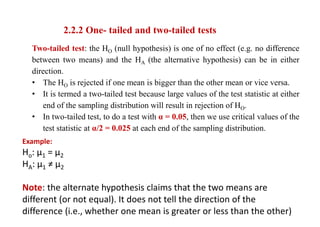
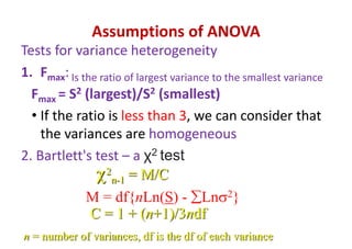
182. Main effects are the averages of the simple
effects
• A main effect is the effect of an independent variable on a
dependent variable averaging across the levels of any other
independent variables.
• It is the average of the simple effects of a given independent
variable
From the above example,
• Main effect of variety = ½ (Simple effect of A at bo + Simple
effect of A at b1)
= ½ [(a1b0-a0b0) + (a1b1-a0b1)] = ½ [(2-1) + (4-1)] = 2
• Main effect of nitrogen = ½ (Simple effect of factor B at ao +
Simple effect of factor B at a1) = ½ [(a0b1-a0b0) + (a1b1-a1b0)] =
½ [(1-1) + (4-2)] = 1

183. Interaction
• Sometimes the factors act independent of each other. By this we mean
that changing the level of one factor produces the same effect at all levels
of another factor.
• However, the effects of two or more factors are not independent in most
cases.
• Interaction occurs when the effect of one factor changes as the level of
the other factor changes (i.e., the impact of one factor depends on
the level of the other factor).
 e.g. if the effect of 50kg N on variety X is 10 Q/ha and its effect on a
variety Y is 15 Q/ha, then there is interaction.
• if there is no interaction it is concluded that the factors under
consideration act independently of each other.
• When interaction effects are present, interpretation of the
main effects is misleading.

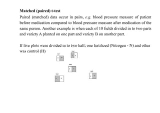
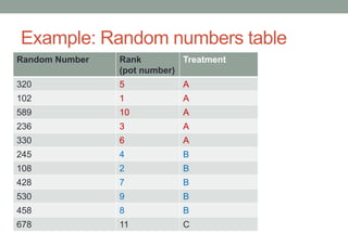
184. Interaction
• Interaction is calculated as the average of the difference
between the simple effects.
• From the above example, it is calculated as the average of
the difference between simple effects of A at the two levels of
B or the difference between the simple effects of B at the two
levels of A.
= ½ (Simple effect of A at b1 – simple effect of A at b0)
= ½ [(a1b1-a0b1) - (a1b0-a0b0)] = ½ [(4-1) - (2-1)] = 1
OR
= ½ (Simple effect of B at a1 – simple effect of B at a0)
= ½ (a1b1-a1b0) - (a0b1-a0b0)] = ½ [(4-2) - (1-1)] = 1

185. Types of Interaction

186. Cross-over
interaction/high
interaction/qualitative
interaction
Quantitative
interaction/non-
cross-over

187. Assignment of Experimental Units:
Assume we have 2 factors. Factor A has three levels a1 , a2 and a3 and factor
B has three levels b1, b2, and b3 then the layout of the completely
randomized design is as follows:
a1b1 a1b2 a1b3 a2b1 a2b2 a2b3 a3b1 a3b2 a3b3
y111
y112
y113
…
y11n
y121
y122
y123
…
y12n
y131
y132
y133
…
y13n
y211
y212
y213
…
y21n
y221
y222
y223
…
y22n
y231
y232
y233
…
y23n
y311
y312
y313
…
y31n
y321
y322
y323
…
y32n
y331
y332
y333
…
y33n
Total sample is nab = n(3)(3) randomly assigned to the different
combinations, n=number of replications
Factorial experiment in Completely Randomized Design

190. Example of a 2x2 factorial
experiment in CRD
Factor A= Nitrogen with 0 and 50kg/ha
Factor B= Phosphorus with 0 and 25kg/ha
Dependent variable= pods per plant (ppp) of
common bean
No.of replications=4

191. Raw Data
1. Summarize the raw data based on treatment combinations and
calculate the treatment total (Tij) and grand total (Gijk) (above table)
Treatment
a0b0 a0b1 a1b0 a1b1
12 19 29 32
15 22 27 35
14 23 33 38
13 21 30 37
Treatment Total Tij 54 85 119 142 Gij = 400
2. Calculate correction factor (C.F) and Total Sum of Squares
(TSS) from the above table
C.F.= Gij
2 /abr = 4002/2*2*4= 160,000/16= 10,000
where a= level of factor A, b=level of factor b and r= number of replications

192. •4. From the above table, calculate treatment sum of square (SSt), Factor
A Sum of Square (SSA), Factor B Sum of Squares (SSB), Factor A x
Factor B Interaction Sum of Squares (SSAxB), and Sum of Square of Error
(SSE)

193. Factor B
Factactor A b0 b1 A Total (Ai)
a0 54 85 139
a1
119 142 261
B Total (Bj) 173 227 G = 400
3. Make a two-way table between Factor A and Factor B using the
treatment totals from the above table and calculate Factor A
Total (Ai) and Factor B total (Bj)

194. 5. Summarize the analyses results in ANOVA table and test the
significance of the effects
Source of
variation
df SS MS F-cal. F-tab.
5% 1%
Treatment ab-1=3 1116.50
 Factor A a-1=1 930.25 930.25 208.65** 4.75 9.33
 Factor B b-1=1 182.25 182.25 40.88** 4.75 9.33
 AxB (a-1)(b-1)=1 4.00 4.00 0.90ns 4.75 9.33
Error ab(r-1)=12 53.50 4.46
Total abr-1=15 1170.00

195. Interpretation

197. The ANOVA Procedure
Class Level Information
Class Levels Values
Trt 4 1 2 3 4
A 2 a0 a1
B 2 b0 b1
Number of observations 16

198. data CRDfactorial;
input Trt A$ B$ Rep PPP;
cards;
1 a0 b0 1 12
1 a0 b0 2 15
1 a0 b0 3 14
1 a0 b0 4 13
2 a0 b1 1 19
2 a0 b1 2 22
2 a0 b1 3 23
2 a0 b1 4 21
3 a1 b0 1 29
3 a1 b0 2 27
3 a1 b0 3 33
3 a1 b0 4 30
4 a1 b1 1 32
4 a1 b1 2 35
4 a1 b1 3 38
4 a1 b1 4 37
;
Proc ANOVA;
Class Trt A B;
Model PPP= A B A*B;
Means A B/Tukey;

199. Dependent Variable: PPP
Sum of
Source DF Squares Mean Square F Value Pr > F
Model 3 1116.500000 372.166667 83.48 <.0001
Error 12 53.500000 4.458333
Corrected Total 15 1170.000000
R-Square Coeff Var Root MSE PPP Mean
0.954274 8.445906 2.111477 25.00000
Source DF Anova SS Mean Square F Value Pr > F
A 1 930.2500000 930.2500000 208.65 <.0001
B 1 182.2500000 182.2500000 40.88 <.0001
A*B 1 4.0000000 4.0000000 0.90 0.3622

200. Tukey's Studentized Range (HSD) Test for PPP
NOTE: This test controls the Type I experiment wise error rate, but it
generally has a higher Type II error rate than REGWQ.
Alpha 0.05
Error Degrees of Freedom 12
Error Mean Square 4.458333
Critical Value of Studentized Range 3.08132
Minimum Significant Difference 2.3003
Tukey Grouping Mean N A
A 32.625 8 a1
B 17.375 8 a0
Tukey Grouping Mean N B
A 28.375 8 b1
B 21.625 8 b0

201. Level of Level of -------------PPP-------------
A B N Mean Std Dev
a0 b0 4 13.5000000 1.29099445
a0 b1 4 21.2500000 1.70782513
a1 b0 4 29.7500000 2.50000000
a1 b1 4 35.5000000 2.64575131
Interaction means

202. Factorial in RCBD
Example: An agronomist wanted to study the effect
of different rates of phosphorus fertilizer on two
varieties of common bean (two-factorial experiment
in RCBD) with four replications
• Variety: two levels (T1 = Indeterminate,
T2 = Determinate)
• Phosphorus rate: 3 levels (P1 = none,
P2 = 25 kg/ha, P3 = 50 kg/ha).
• Six treatment combinations: T1P1; T1P2; T1P3;
T2P1; T2P2; T2P3

203. Field layout and yield of common bean (Q/ha)

204. The linear model for Two Factor Randomized Block Design:
Yijk =  + i + j + k + ik + ijk
where, Yijk = the value of the response variable;  = Common
mean effect; i = Effect of factor A; j = Effect of block; k = Effect
of factor B; ik = Interaction effect of factor A & factor B; and ijk
= Experiment error (residual) effect

209. Interpretation
Since A  B interaction is highly significant, the results of
experiment are best summarized in a two way table of means of A
 B combinations.
Note: when interaction is not significant, all of the information in
the trial is contained in the significant main effects.
• In that case the results may be summarized in tables of mean for
factors with significant main effects.

210. Variety  Phosphorus rate means

211. Chapter 6: Split-Plot Design

212. Split-plot design
• It involves two different plot sizes (main plot and sub-
plot).
• The levels of one factor (i.e., main plot factor) are assigned
at random to large experimental units (main plots).
• The large units are then divided into smaller units (sub-
plots)
– then the levels of the second factor (i.e., sub-plot
factor) are assigned at random to the sub-plots
within the main plots.
• The large units are called the whole units or main-plots
whereas the small units are called the split-plots or sub-plots
(units).

213. • In split-plot design, the main plot factor effects
are estimated from the larger units, while the sub-
plot factor effects and the interactions of the main-
plot and sub-plot factors are estimated from the
small units.
• As there are two sizes of experimental units, there
are two types of experimental error, one for the
main plot factor and the other for the sub-plot
factor.
• the error associated with the sub-plots is smaller
than that for the main plots due to the fact that error
degrees of freedom for the main plots are usually
less than those for the sub-plots.

214. Guidelines to apply factors either to
main-plots or sub-plots:
a. Degree of precision required: Factors which require
greater degree of precision should be assigned to the sub-
plot.
• For example, animal breeder testing three breeds of dairy
cows under different types of feed stuff may assign the
breeds of animals to sub-units and the feed stuffs to the
main unit.
• On the other hand, animal nutritionist may assign the feeds
to the sub-units and the breeds of animals to the main-units
as he is more interested on feed stuffs than breeds.
What is the reason?

215. b. Relative size of the main effect: If the main effect of one factor
(factor A) is expected to be much larger and easier to detect than
factor B, then factor A can be assigned to the main unit and factor
B to the sub-unit.
• For instance, in fertilizer and variety experiments, the researcher
may assign variety to the sub-unit and fertilizer rate to the main-
unit, because he expects fertilizer effect to be much larger and
easier to detect than the varietal effect.
c. Management practice: The factors that require smaller
experimental area (plot) should be assigned to sub-plots.
• For example, in an experiment to evaluate the frequency of
irrigation (5, 10, 15 days) on performance of different tree
seedlings on nursery, the irrigation frequency factor could be
assigned to the main plot and the different tree species to the
sub-plots to minimize water movement to adjacent plots.
 What does this mean?

216. Randomization and layout
• There are two separate randomization process in
split-plot design, one for the main plot factor and
another for the sub-plot factor.
• In each block, the main plot factors are first
randomly applied to the main plots followed by
random assignment of the sub-plot factors.
• Each of the randomization is done by any of the
randomization schemes.

217. Procedures of randomization
Step 1: Divide the experimental area into r blocks,
and divide each block into a main plots.
• Then randomly assign the levels of the main plot
factor to the main plots in each of the blocks.
• Note that the arrangement of the main-plot factor
can follow any of the designs: CRD, RCBD and
LATIN square.
Step 2: Divide each of the main plot (unit) in to b
sub plots and randomly assign the levels of the sub-
plot factor to the sub-plot in each main plot .

218. Note:
• Each main-plot factor is tested r-times where r is
the number of blocks while each sub-plot factor is
tested a  r times where a is level of factor A and r
is the number of blocks.
 This is the primary reason for more precision for
the sub-plot factors as compared to the main-plot
factors.

219. Example: An experiment was designed to test the effect of
feeding four forage crops (Rhodes grass, Vetch, Alfalfa and Oat)
on weight gain (kg/month) of two breeds of cows (Zebu,
Holstein).
• At the start of the experiment, it was assumed that breeds of
cows would respond differently to the feed stuffs.
• The objective of the experiment was to compare the effect of
forage crops as precisely as possible.
• Therefore, the experimenter assigned the breeds of animals to
the main-plot and the four forage crops to the sub-plots.
• The experiment was replicated in three blocks (barns) based
on initial body weight of animals as a blocking factor.

220. - Main-plot factor is breed of animals: Holstein (H), Zebu (Z).
- Split-plot (units) factor is feed stuffs: Alfalfa (A), Vetch (V),
Rhodes grass (R), Oat (O)
Main
plot
Sub-plot

221. Analysis of variance
The linear model for Split Plot Design:
Yijk =  + i + j + k + ()ij + ()ik + ijk
where, Yijk = the value of the response variable;
 = Common mean effect;
i = Effect of factor A (main plot factor);
j = Effect of block;
k = Effect of factor B (sub-plot factor);
()ij= Interaction effect of factor A & Block (errora);
ik = Interaction effect of factor A & B
ijk = Experiment error (residual) effect (errorb)

222. Steps of Analysis
Step 1: Arrange data by treatments (main-plot, sub-plot) and blocks and
calculate main-plot total, and sub-plot total.
Treatments Blocks
Breeds Feeds I II III
Holstein Alfalfa 25.9 26.7 27.6
Vetch 25.3 24.8 28.4
Oat 19.3 18.0 20.5
Rhodes grass 22.2 24.2 25.4
Main-plot totals 92.7 93.7 101.9
Zebu Alfalfa 18.9 18.3 19.6
Vetch 21.0 22.7 22.3
Oat 13.8 13.5 13.2
Rhodes
grass
15.5 15.0 15.2
Main-plot totals 69.2 69.5 70.3

223. Step 2: Construct two way tables of totals.
2.1. Block by factor A two-way table and compute block total, factor A
total and grand total.
Weight gain totals of block by factor A.
Breeds (A) Block 1 Block 2 Block 3 Factor A (breeds)
total
Holstein 92.7 93.7 101.9 288.3
Zebu 69.2 69.5 70.3 209.0
Block total 161.9 163.2 172.2
Grand total 497.3 = G
2.2. Factor A by factor B total two-way table and calculate factor B totals
Breeds (A) Alfalfa
(b1)
Vetch
(b2)
Oat (b3) R. Grass
(b4)
Holstein (a1) 80.2 78.5 57.8 71.8
Zebu (a2) 56.8 66.0 40.5 45.7
Factor B total 137.0 144.5 98.3 117.5

224. Values in Factor A x
Block table (table 2.1)

225. SS of treatment

226. RCBD repeated
“a” times

227. Step 7: Construct the ANOVA Table, obtain the corresponding tabulated F-
value and compare it with the calculated F-value at prescribed level of
significance.
Source of
variation
D.F. SS MS Calculate
d
F-value
Tabulated F
5% 1%
Block (r-1) = 2 7.87 3.93 1.56ns 19.0 99.0
Breeds (A) (a-1) = 1 262.02 262.02 104.39** 18.51 98.5
Error (a) (r-1) (a-1) = 2 5.03 2.51
Feeds (B) (b-1) = 3 215.26 71.75 119.58** 3.49 5.95
A  B (a-1) (b-1) = 3 18.70 6.23 10.38** 3.49 5.95
Error (b) a(r-1)(b-1) = 12 7.24 0.60
Total (rab-1) = 23 516.12

228. Remark: Since Interaction is highly significant, a two-way table of Factor A
and Factor B means should be presented with appropriate mean
separation test (see next slide)

229. Mean weight (kg/month) of Holstein and Zebu breeds fed with four types of
forage species
Breeds (A) Alfalfa
(b1)
Vetch
(b2)
Oat (b3) R. Grass
(b4)
Factor A
mean
(A total/rb)
Holstein (a1) 26.7 26.2 19.3 23.9 24.0 (A1)
Zebu (a2) 18.9 22.0 13.5 15.2 17.4 (A2)
Factor B
mean
(B total/ra)
22.8 (B1) 24.1 (B2) 16.4 (B3) 19.6 (B4)
Grand mean
= 20.72
Conclusion:
• For Holstein cows, feeding alfalfa results in higher weight gain/month.
However, vetch can also be used as a substitute for alfalfa when the latter is
not available, with almost similar effect on weight gain.
• For the Zebu cows, feeding vetch results in the highest weight gain/month.
However, the use of alfalfa could also be considered when the former is in
short supply.

230. • Since the mean difference (d) between B2 and B3 (24.1 – 16.4 = 7.7) is
greater than LSD value at 1% (1.37), the difference between the two means
is highly significant.

233. Chapter 7: STRIP-PLOT DESIGN

234. Strip-Plot Design
• The strip-plot design is specifically suited for a two-factor
experiment in which the desired precision for measuring the
interaction effect between the two factors is higher than that
for measuring the main effect of either one of the two
factors.
This is accomplished with the use of three plot sizes:
1. Vertical strip plot for the first factor – vertical factor
2. Horizontal strip plot for the second factor – horizontal
factor
3. Interaction plot for the interaction between 2 factors

235. • The vertical-strip plot and the horizontal-strip plot are
always perpendicular to each other.
• In strip plot design, each block or replication is divided into
number of vertical and horizontal strips depending on the
levels of the respective factors.
• There is no relationship between the sizes of the
vertical and horizontal strip plots, unlike the case
of main plot and subplot of the split-plot design.
• The interaction plot is the smallest and provides
information on the interaction of the 2 factors.
• The interaction is tested with more precision in strip plot
design.

236. S= Vertical factor
N= Horizontal factor
Interaction plot

237. Randomization and Layout
• The procedure for randomization and layout
of a strip-plot design consists of two
independent randomization processes-one
for the horizontal factor and another for the
vertical factor
• The order in which these two processes are
performed does not matter.

238. • Let A represent the horizontal factor and B the vertical
factor, and a and b their levels, while r represents the
number of replications.
• Here, a two-factor experiment involving six rice
varieties (horizontal treatments) and three nitrogen
rates (vertical treatments) tested in a strip-plot design
with three replications is illustrated.
STEP 1. Assign horizontal plots by dividing the
experimental area into r = 3 blocks and dividing each of
those into a = 6 horizontal strips.
• Follow the randomization procedure for a randomized
complete block design with a = 6 treatments and r = 3
replications and randomly assign the six varieties to the six
horizontal strips in each of the three blocks, separately and
independently.

239. STEP 2. Assign vertical plots by dividing each block in to
b = 3 vertical strips.
• Follow the randomization procedure for a randomized
complete block with b = 3 treatments and r = 3
replications and randomly assign the three nitrogen
rates to the three vertical strips in each of the three
blocks, separately and independently.

240. Analysis
The analysis is carried out in 3 parts.
1. Vertical strip analysis
2. Horizontal strip analysis
3. Interaction analysis
 When there are r replications, a levels for factor A and
b levels for factor B, then the ANOVA table is as
shown below.
SV

241. Example:
Data
on
Grain
Yield
of
Six
Varieties
of
Rice,
Grown
with
Three
Nitrogen
Rates
In
a
Strip-
plot
Design
with
Three
Replications)

242. Analysis of Variance procedure for data from a two-factor experiment
involving six rice varieties (horizontal factor) and three nitrogen levels
(vertical factor) tested in three replications.

243. STEP 2. Construct three tables of totals:
1. The replication x horizontal-factor table of totals with
replication totals, horizontal-factor totals, and grand total
computed.

253. ANOVA Table

255. 8.0. Combine Analysis of Data

256. • In field experiments, it is necessary to repeat the experiments over a number of
locations, seasons, or both, e.g. varietal trials, plant spacing, fertilizer trials.
• The purpose of repeating the experiments is to find recommendation that can
be applied over space (location), time (season) or both.
• In such repeated experiments, appropriate statistical procedures for a combined
analysis of data have to be used.
The main purposes of combined analysis of data are:
 to estimate the average response over a wide range of environments
 to test the consistency of the response from place to place or year to year, i.e. to
determine if there is interaction effect of the treatments, e.g. stability analysis
of varieties.
 If the response is consistent from place to place and year to year, it shows the
absence of interaction.

257. 1. Construct an outline of combined analysis over years or locations or both on
the basis of experimental design used.
Steps of combined analysis
 For example, the outline of ANOVA for the experiment conducted at six
environments with five treatments and six replications in RCBD is given as:
___________________________________________________________________
Source Degrees of
freedom Mean squares Computed F
________________________________________________________________________
Environment (E) (e-1) = 5 EMS EMS/RMS
Blocks/within environment e(r-1) = 30 RMS
Treatments (T) (t-1) = 4 TMS TMS/MSE
T x E (e-1) (t-1) = 2 ExTMS E xTMS/MSE
Pooled error e(r-1) (t-1) = 120 MSE
________________________________________________________________________
Where e = no. of environments; r = no. of replications; t = no. of treatments; EMS = environment
mean square; RMS is blocks/replications mean square; TMS = treatment mean squares; and MSE =
mean square error.

258. 2. Compute the usual ANOVA for each environment according to RCBD and
obtain the mean squares of error and degrees of freedom from individual
environment analysis.
________________________________________________________________________
Environment: E1 E2 E3 E4 E5 E6
Error d.f. (r-1)(t-1) 20 20 20 20 20 20
Error MS 5776 4028 4516 9526 7056 5535
________________________________________________________________________
3. Test the homogeneity of the variances
Case 1: When there are only two environments, use F-test as:
F calculated = and compare with table F-value at d.f. for larger
error mean square as numerator and d.f. for smaller error mean square as
denominator.
If F-calculated is > F-table, the null hypothesis of homogeneity of variances is
rejected, i.e. the error variances are heterogeneous. Thus, combined analysis
conducted directly. We can analyze the data separately or transform the data to
homogenize the error variances to use combined analysis.
 On the other hand, if the F-calculate value is ≤F-table, the error variances are
homogeneous, thus we can directly proceed to combined analysis.

259. Case 2: When environment is more than two, use Bartlett’s chi-square test
2
c =
)
1
1
)(
)
1
(
3
1
(
1
)
log
log
(
3026
.
2
1










kj
kj
e
MSEi
kj
MSE
kj
k
i
Where
Kj = Error d.f. for each environment

MSE = Pooled error mean square = = = 6072.83
MSEi = Error mean square for each environment
e = number of environment
Environment Kj MSE log MSE Kj x MSE Kj x log MSEi 1/kj
E1 20 5776 3.761627 75.6 75.23254 0.05
E2 20 4028 3.605089 75.6 72.10179 0.05
E3 20 4516 3.654754 75.6 73.09508 0.05
E4 20 9526 3.978911 75.6 79.57821 0.05
E5 20 7056 3.848559 75.6 76.97117 0.05
E6 20 5535 3.743118 75.6 74.86235 0.05
453.6 451.8411 0.3

MSE = Pooled error mean square = =
= 6072.83
Log (6072.83) = 3.78
2
c =
)
008
.
0
3
.
0
)(
)
5
(
3
1
(
1
)
84
.
451
6
.
453
(
3026
.
2



; 2
c = 3.97
2
(e-1) 5% = 2
c (5) 5% = 11.07,
Since 2
c (3.97) is less than 2
table at 5% (11.07), accept the null hypothesis. Thus, this
• Since 2c (3.97) is less than 2 table at 5%
(11.07), accept the null hypothesis. Thus, this
implies the errors are homogeneous. Hence,
combined analysis an be conducted using the
appropriate model.

260. ANOVA MODELS
Fixed, Random, Mixed

261. ANOVA MODELS and EXPECTED MEAN SQUARES
there will be an additional component in the variance

262. different

271. Chapter 9: COMPARISON OF
TREATMENT MEANS

272. • The F-test (ANOVA) shows whether there is significant difference
among treatments or not. We have to conduct mean separation test
(mean comparison) to know the specific treatment pairs that are
significantly different.
• There are many ways to compare the means of treatments tested in an
experiment. One of these is pair comparison, which is the simplest and
most commonly used comparisons in agricultural research.
There are two types of pair comparisons:
A. Planned pair comparison: In which the specific pair of treatments to be
compared are identified before the start of the experiment, e.g. comparing
the control treatment with each of the other treatments- A priori test
B. Unplanned pair comparison: In which no specific comparison is
chosen in advance. Instead, every possible pair of treatment means are
compared to identify pairs of treatments that are significantly different,
e.g. variety trials. A posteriori test or Post hoc test

273. The most commonly used test procedures for pair
comparison in agricultural research are:
 the Least Significant Difference (LSD) and Tukey’s
test which are suitable for planned pair comparison,
and
 Duncan’s Multiple Range Test (DMRT) which is
applicable to an unplanned pair comparison.
9.1. Least Significant Difference (LSD) Test
• LSD is the simplest and the most commonly used procedure for making
pair comparisons.
• The procedure provides a single value at a prescribed level of
significance, which serves as the boundary between significant and non-
significant differences between any pair of treatment means.
• That is, two treatments are declared significantly different at a
prescribed level of significance if their mean difference exceed the
computed LSD value, otherwise they are not significantly different.

274. Remark:
• The LSD test is not valid for comparing all possible pair of means,
especially when the number of treatments is large.
• This is so because, in experiments where no real difference exists
among all treatments, the numerical difference between the largest
and smallest treatment means is expected to exceed the LSD value
when the number of treatments is large
• To avoid this problem, the LSD test is used only when the F-test for
treatment effect is significant and the number of treatments is not too
large (less than six).

275. The procedure for applying the LSD test to compare any two treatments
means
1. Rank the treatment means from the largest to the smallest in the column and
from the smallest to largest in rows.
2. Compute all possible differences between the two treatment means to be
compared.
3. Compute the LSD value at α level of significance
LSDα = tα/2 (n)  sd
where sd = standard error of the treatment mean difference; tα/2 (n) is the table t-
value at α/2 level of significance and with n error degree of freedom

276. N
o
Treatments (stage of application of
N)
Treatment
mean (g)
1 Seedling 5.10
2 Early blooming 4.30
3 Half blooming 4.00
4 Full Blooming 6.70
5 Ripening 6.05
6 Unfertilized (control) 7.03
Example: Oil content (g) of linseed treated at different six stages of growth with N-
fertilizes tested in RCBD in four replications with error mean square of 1.31.
LSD5% = t0.025(15)  r
MSE
2
, where MSE is error mean square; r is the number
of replications = 2.131  

4
31
.
1
2
1.72 g
LSD1% = t 0.005(15)  r
MSE
2
= 2.947  g
39
.
2
4
31
.
1
2



277. Treatments 4.00
(T3)
4.30
(T2)
5.10 (T1) 6.05 (T5) 6.70 (T4) 7.03
(T6)
7.03 (T6) 3.03** 2.73** 1.93* 0.98ns 0.33ns -
6.70 (T4) 2.70** 2.40** 1.60ns 0.65ns -
6.05 (T5) 2.05* 1.75* 0.95ns -
5.10 (T1) 1.10ns 0.80ns -
4.30 (T2) 0.30ns -
4.00 (T3) -
4. Compare the mean difference (d) in step 2 with LSD value computed in step (3) using the
following rule:
 if /d/ >LSD value at 1% level of significance, there is highly significant difference between the
two treatment means compared (put two asterisks on differences).
 if /d/>LSD value at 5% level of significance but < LSD value at 1% level of significance, there is
significant difference between the two treatment means compared (put one asterisks on
differences)
 if /d/  LSD value at 5% level of significance, the two treatment means compared are not
significantly different (put n.s.)
Note that there are
2
)
1
( 
t
t
possible (unplanned) pair comparisons and (t-1) planned pair
comparisons where t is the number of treatments. In the above example, 15 unplanned
pair comparisons and five planned pair comparisons are possible, since we have one
control.

278. • The differences between T6 & T3, T6 & T2, T4 & T3, T4 & T2 are
highly significant; while the differences between T3 & T5, T1 & T6, T2
& T5 are significant.
Presentation of data using LSD
Table __. Mean oil content of linseed treated with
nitrogen fertilizer at different stages
___________________________________________
Stage of application Oil content (g)
___________________________________________
Seedling 5.10
Early blooming 4.30
Half-blooming 4.00
Full- blooming 6.70
Ripening 6.05
Unfertilized 7.03
___________________________________________
LSD(0.05) 1.72 g
CV (%) 20.7

279. 9.2 Duncan’s Multiple Range Test (DMRT)
• It is most widely used to make all possible pair comparisons.
• The procedure for applying the DMRT is similar to LSD test but
it requires progressively larger values for testing significance
between the treatment means as they are more widely
separated in the array.
 i.e., it requires multiple critical values unlike a single value in
LSD
• The test is more appropriate when the total number of
treatments is large.
• It involves the calculation of the shortest significant difference
(SSD).
• The SSD is calculated for all possible relative positions (P)
between the treatment means when the means are arranged in
order of magnitude (in decreasing or increasing order).

280. Procedure
Step 1: Arrange all the treatment means in increasing or decreasing order.
• Data such as crop yield are usually arranged from the highest to the
lowest.
Example: Yields (kg/plot) of wheat varieties grown in 4 x 4 Latin Square
Design with error mean square of 0.45:
B (12.3), A (12.00), C (10.8), D (6.7)
Step 2: Calculate (the standard error of the treatment mean difference) as:
r
MSE
d
s
2
 = kg
d
s 47
.
0
4
45
.
0
2




281. Step 3: Calculate the shortest significant difference (SSD) for relative positions
(P) in the array of means.
Since we have four treatment means, they can be 2, 3 and 4 distance apart.
B and A are 2 distance apart (P = 2); B and C are 3 distance apart (P = 3);
B and D are 4 distance apart (P = 4); A and D are 3 distance apart (P =
3); etc.
For the above example, the R values with error d. f. of 6 at 1% level of
significance are found from R-table (see Appendix F in Gomez & Gomez)
P = 2 3 4
R0.01 = 5.24 5.51 5.65
SSD = 1.74 1.83 1.88
P = the distance in ranks between the pairs of treatment means to be compared.
R= significant studentized range at error d. f. (6).
SSD (Shortest Significant Difference) = 2

 sd
R
SSD at P = 2 = 74
.
1
2
47
.
0
24
.
5


SSD at P = 3 = 83
.
1
2
47
.
0
51
.
5


SSD at P = 4 = 88
.
1
2
47
.
0
65
.
5


 Note that SSD values increase as the distance between treatments (P) to be
compared increases.

282. Step 4: Test the difference between treatment means in the following
order.
 Largest – Smallest = 12.3 – 6.7 = 5.6; compare with SSD value at (P = 4) = 1.88; d
(5.6) > SSD at P = 4 (1.88); thus the difference is significant at 1% level of
significance.
 Largest – 2nd smallest = 12.3 – 10.8 = 1.5; compare with SSD at (P=3) = 1.83; d
(1.5) < SSD at P= 3 (1.83); thus, the difference is non-significant at 1% level of
significance.
 Largest – 2nd largest = 12.3 – 12.0 = 0.3 < SSD at P = 2 (1.74); thus, the difference
is non-significant at 1% level of significance.
 2nd largest – smallest = 12.0 - 6.7 = 5.3; compare with SSD at P = 3 (1.84); d (5.3) >
SSD (1.84) at P = 3; significant at 1% level of significance
 2nd smallest – smallest = 10.8 – 6.7 = 4.1 compared with SSD at P = 2 (1.74); d
(4.1) > SSD (1.74) at P = 2; significant
 etc
Note that SSD value at (P=2) is equals to LSD value

283. ________________________________________________________
B (12.3) A (12.0) C (10.8) D (6.7)
_____________________________________________
D (6.7) 5.6**
(P=4) 5.3**
(P=3) P = 4.1**
(P=2) -
C (10.8) 1.5ns
(P=3) 1.2ns
(P=2) -
A (12.0) 0.3ns
(P=2) -
B (12.3) -
________________________________________________________
SSD (P = 4) = 1.88; SSD (P =3) = 1.83; SSD (P =2) = 1.74
Treatments B & D, A & D, C & D are significantly different at 1%, while treatments B &
C, B & A, and A & C are not significantly different at 1% level of significance.

284. Step 5: Present the test result in one of the following two ways
A. Use a line notation if the sequence of results can be arranged according
to their ranks.
 Any two means underscored by the same line are not significantly
different at 1% level of significance according to DMRT.
B(12.3) A(12.0) C(10.8) D(6.7)
B. Use the alphabet notation if the desired sequence of the results is not
based on their rank which is commonly used.
 The alphabet notation can be derived from line notation simply by
assigning the same alphabet to all treatment means connected by the
same horizontal line.
 It is usual practice to assign letter a for the first line, b for the second
line, c for third line and so on.
 Note that letter a can be used for the largest or smallest treatment mean
depending on the rank of arrangement.

285. Presentation of data using DMRT
Table __ Mean yields of wheat varieties planted at Debrezeit Agricultural Research
Center.
Variety Yield
(kg)
A 12.0 a
B 12.3 a
C 10.8 a
D 6.7 b
Note that we have to put a footnote below the table stating that any two means in the
same column followed by the same letter are not significantly different at 1% level of
significance according to DMRT. Note also that both LSD and DMRT are not used in
the same table. Use either of them depending on the appropriateness of the test.

286. 8.3 Tukey’s Test
 It is more conservative than LSD test because it requires the largest treatment mean
differences for significance.
It is computed in a manner similar to the LSD test except that standard error of
the mean is used instead of standard error of the mean difference ( d
s ), and
Studentized range (q-table) is used in place of t-table
The procedure:
1. Select a value from q table, which depends on the number of means (n) and error
degree of freedom (v).
2. Compute the Critical Difference (CD) as = q(n, v) 
r
MSE
where MSE is error mean
square; n is number of means to be compared; v is error degrees of freedom and
r is number of replications.
3. For any pair of means, if the absolute value of the difference /d/ > critical value, the
difference is judged to be significant at a prescribed level of significance.

287. Example: The following analysis of variance table is from CRD with six varieties
replicated four times in glass house (mean rust incidence)
__________________________________________________________Source d. f.
MS F-cal. F-table (5%)
____________
Variety (t-1) = 5 2976.44 24.80** 2.77
Error t(r-1) = 18 120.00
__________________________________________________________
Variety: 1 2 3 4 5 6
Mean stem rust incidence (%): 50.3 69.0 24.0 94.0 75.0 95.3
n= 6; V= 18; q0.05 (6, 18) = 4.495
CD = q  r
MSE / = 4.495 
4
120
= 24.62%

288. Difference between means
________________________________________________________________________
24.0(3) 50.3(1) 69.0(2) 75(5) 94(4) 95.3(6)
_________________________________________________________
95.3(6) 71.3* 45.0* 26.3* 20.3ns
1.3ns
-
94(4) 70.0* 43.7* 25.0* 19.0ns
-
75(5) 51.0* 24.7* 6.0ns
-
69(2) 45.0* 18.7ns
-
50.3(1) 26.3* -
24.0(3) -
________________________________________________________________________
Thus, differences between varieties 6&3, 4&3, 5&3, 2&3, etc. are significant while differences between varieties
2&1, 5&2, etc. are non-significant.
READ: 8.4. Pair Comparisons with Missing Data

289. 10.0 ANALYSIS OF COVARIANCE

290. • The analysis of covariance simultaneously examines the variance and
covariance of selected variables so that the character of primary interest is
more accurately characterized than by the use of analysis of variance only.
• Analysis of covariance requires measurement of the character of interest
(variate) and the measurement of one or more variable(s) known as
covariate(s).
• It also requires that the functional relationship of the co-variates (x) with the
character of primary interest (y) is known before hand (i.e., they should be
correlated).
Examples: Consider wheat variety trial in which weed infestation is used as a
co-variate with a known functional relationship between weed incidence and
grain yield (the character of primary interest), the covariance analysis can adjust
grain yield in each plot to a common level of weed infestation.
 With the covariance analysis, the variation in yield due to weed infestation
is quantified and effectively separated from that due to varieties.

291. 10.1 Uses of Covariance Analysis
1. To Control Experimental Error
• One way to reduce experimental error is by using proper type of blocking.
• However, blocking can not cope with certain types of variability such as spotty
soil heterogeneity and unpredictable insect/disease incidence.
 In such cases, heterogeneity between experimental plots does not follow a
definite pattern, thus blocking is not possible.
 By measuring an additional variable (i.e covariate) that is known to be linearly
related to the primary variable (y), the source of variation associated with the
covariate can be deducted from experimental error.

292. 2. Adjustment of Treatment Mean
• With the covariance analysis, the primary variable (y) can be adjusted
linearly up wards or down wards depending on the relative size of its
respective covariate (x).
• The treatment mean of the dependent variable is adjusted to a value that it
would have had there been no differences in the value of the co-
variate. e.g. number of plants harvested per plot, age of cows, initial body
weight of the cow, etc.
Remark: In situations where real differences among treatments for the
independent variable do occur but are not the direct effect of the
treatments, adjustment is warranted, e.g. in variety trial, if seeds may differ
widely in germination, not because of inherent differences of the varieties,
adjustment can be done, but if the density is treatment by itself there is no
need to adjust the means.

293. 3. Interpretation of Experimental Results
Covariance analysis aids the experimenter in understanding the principles
underlying the results of an investigation.
• By examining the primary character of interest (y) together with other
characters (x) whose functional relationship to y are known, the biological
process governing the treatment effects on y can be characterized more
clearly.
4. Estimation of Missing Data
The missing data formula technique biases the treatment sum of squares
upwards.
 The use of covariance analysis to estimate the missing value(s) results in a
minimum residual sum of squares and unbiased treatment sum of squares.

294. 9.2. Computation Procedure
• Covariance analysis is an extension of analysis of variance.
 It is a combination of analysis of variance and linear regression.
• Covariance analysis can be used for CRD; RCBD and split-plot designs, but
the computation procedures vary some what.
Computation procedure for RCBD
The following data show ascorbic acid content (y) of ten varieties of common
bean.
• From previous experiences, it was known that increase in maturity resulted
in decrease in vitamin C content (linear r/ship)- Inverse r/ship.
• Since all varieties were not at the same level of maturity on the same day, it
was not possible to harvest all plots at the same stage of maturity.
• Hence, the percentage of dry matter based on 100 g of freshly harvested
beans was observed as an index of maturity and used as a covariate.

295. Ascorbic acid content (ASAC, mg/100 g of seed) and percentage of dry matter (% DM) for common bean varieties
___________________________________________________________
Block I Block 2 Block 3
____________ _____________ ______________
Variety % DM ASAC % DM ASAC % DM ASAC
____________________________________________________________
1 34 93 33 95 35 92
2 40 47 40 51 51 33
3 32 81 30 100 34 72
4 38 67 38 74 40 65
5 25 119 24 128 25 125
6 30 106 29 111 32 99
7 33 106 34 107 35 97
8 34 61 31 83 31 94
9 31 80 30 106 35 77
10 21 149 25 151 23 170
_______________________________________________________________
Conduct the analysis of covariance & calculate standard error of mean
difference

296. Variety Block I Block II Block III Variety total
% DM ASAC % DM ASAC % DM ASAC
X Y X Y X Y X Y
1 34 93 33 95 35 92 102 280
2 40 47 40 51 51 33 131 131
3 32 81 30 100 34 72 96 253
4 38 67 38 74 40 65 116 206
5 25 119 24 128 25 125 74 372
6 30 106 29 111 32 99 91 316
7 33 106 34 107 35 97 102 310
8 34 61 31 83 31 94 96 238
9 31 80 30 106 35 77 96 263
10 21 149 25 151 23 170 69 470
Block
total
318 909 314 1006 341 924 973 2839

297. Steps of Analysis
1. Conduct analysis of variance for each of the variables, covariance and sum of treatment and
error sum of squares
_______________________________________________________________
Source D. F. SS of ASAC (Y) SS of % DM (X) SS of XY
________________________________________________________________
Block 2 545.3 42.47 -75.23
Treatment 9 25689.0 972.70 -4633.23
Error 18 1608.7 86.20 -251.77
Treatment + Error 27 27297.7 1058.90 -4885.00
_________________________________________________________________
2. Analyse covariance
C.F. =
t
r
G
G y
x


=
10
3
2839
973


= 92078.23
Total Sum of Products =  
 .
.F
C
y
x i
i = (34  93) + (40  47) + ... + (23  170) - 92078.23 =
87118-92078.23 = -4960.23
Sum of Products due to Blocks =
t
B
B y
x
 
- C.F.
10
)
924
341
(
)
1006
314
(
)
909
318
( 




- 92078.23 =
92003-92078.23 = -75.23
Sum of Products for Treatments:
r
T
T y
x
 
- C.F. =
3
)
470
69
(
.....
)
131
131
(
)
280
102
( 





- 92078.23 = -
4633.23
Error Sum of Squares of Products = Total Sum of Products – Block SS of Products – Treatment
SS of Products = -4960.23-(-75.23)-(-4633.23)
= -251.77

298. 5. Compute the treatments adjusted SS of Y = Treatment + Error adjusted SS of
Y - Error adjusted SS of Y = 4761.84-873.34 = 3888.5
_____________________________________________________________________
Source D.F SS MS F-cal F table (1%)
_____________________________________________________________________
Treatment (adjust) (t-1) 10-1 = 9 3888.50 432.0 8.41** 3.68
Error (adjusted) (r-1) (t-1)-1= 17 873.34 51.4
____________________________________________________________________

299. 7. Compute adjusted treatment mean as:

Y adjusted = )
(unadjusted
Yi

– b(

i
X – X grand mean).
 For example, for treatment 1=

Y adjusted = 93.33-(-2.921.57)
= 97.92

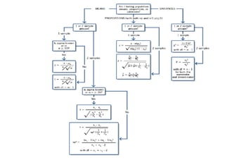
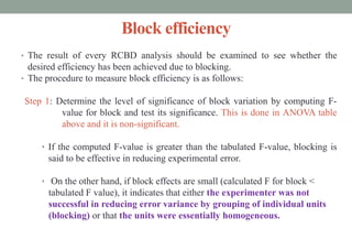
300. Compute the relative efficiency (R.E.) of covariance analysis compared to standard analysis of
variance
R.E. = 100
)
1
)(
(
)
(


X
of
SS
Error
X
of
MS
Treat
Y
of
MS
adjusted
Error
Y
of
MS
unadjusted
Error
100
)
86.2
972.7/9
1
(
)
51.4
(
1608.7/18)
(



 100
115.84
37
.
89

 = 77.15%
 Thus, the result indicates that the use of % dry matter as the covariate has
not increased precision in ascorbic acid content which would have been
obtained had the ANOVA is done without covariance.
CV = 100
x
Y
of
Mean
Grand
Y
of
MS
Error
Adjusted
= 100
94.63
51.4
 = 7.6%
Mean comparison
S

d to compare two adjusted treatment means:
]
)
(
2
[
2
X
of
SS
Error
xj
xi
r
Y
of
Square
Mean
Error
Adjusted

 , where xi & xj are the covariate means of ith
and jth
treatment; r is the number of replications common to both treatments.
 For instance, to compare means of T1 & T2:
S

d = ]
86.2
)
34
-
43.67
(
3
2
[
51.4
2
 where 34 & 43.67 are the covariate means of 1st
and 2nd
treatments;
3 is the number of replications common to both treatments.
S

d = 02
.
90 = 9.49

301. 11. REGRESSION AND CORRELATION ANALYSIS

302. 11.1 Types of Regression & Correlation
• Regression analysis describes the effect of one or more variables (designated
as independent variables) on a single variable (designated as the dependent
variable).
• It expresses the dependent variable as a function of independent variable(s).
 For regression analysis, it is important to clearly distinguish between the
dependent and independent variables.
Examples:
 Grain yield of maize depends on fertilizer rate
 Weight gain in animals depends on feed
 Number of growth rings in a tree depends on age of the tree
In the above cases, weight gain, number of growth rings and grain yield are
dependent variables, while feed, age and fertilizer rates are independent
variables.

303. • The independent variable is designated by x and the dependent variable by y.
 Correlation analysis, on the other hand, provides a measure of the degree of
association between the variables, e.g. the association between height and weight
of students; body weight of cows and milk production; grain yield of maize and
thousand kernel weight.
 No cause-effect r/ship is implied in correlation.
Regression and correlation analysis can be classified:
a. Based on the number of independent variables as:
 Simple: one independent variable and one dependent variable.
 Multiple: if more than one independent variables and a dependent variable
is involved (for regression), or more than one pair of variables are involved
(for correlation)

304. b. Based on the form of functional relationship as:
 Linear: if the form of underlying relationship is linear
 Non-linear: if the form of the relationship is non-linear
• Thus, regression and correlation analysis can be classified into 4:
 Simple linear regression and correlation analysis
 Multiple linear regression and correlation analysis
 Simple non-linear regression and correlation analysis
 Multiple non-linear regression and correlation analysis
Linear Relationships
The relationship between any two variables is linear if the change in y is constant as x
changes through out the range of x under consideration.
• The functional form of linear relationship between a dependent variable y and an
independent variable x is represented by the equation.
y = a + bx
y = is the dependent variable
a = the intercept of the line on the y-axis (the value of y when x is 0)
b = linear regression coefficient, is the slope of the line or the amount of change in y
for each unit change in x.

305. When there are more than one independent variables as say k-independent
variables (x1, x2, ………, xk), the simple linear regression equation y = a +
βx can be extended to the multiple linear functional form of:
y = α + β1x1 + β2x2 +……. + βkxk
where α is the y intercept (the value of y when all x’s are 0); β1, β2, ….. βk
are partial regression coefficients associated with the independent
variables.

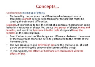
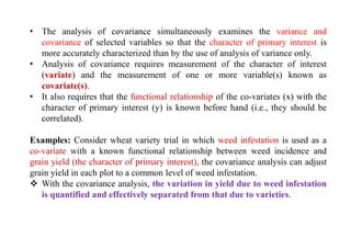
306. 12.2 Simple Linear Regression and Correlation Analysis
12.2.1 Simple linear regression analysis
The simple linear regression analysis deals with the estimation and test of significance
concerning the two parameter α and β in the equation:
Y = α + βx
The data required for the application of the simple linear regression are the n-pairs (with
n >2) of y and x values.
Steps to estimate α and β
Step 1: Compute the means (x and y ), deviation from means [ 
x
x  , 
y
y  ], square of the
deviates (x2
, y2
) and product of deviates (xy).

307. Example: Determine the regression equation for dependence of wing length of 13 sparrows of
various ages.
Age (days),
x
Wing
length
(cm), Y
Deviations from
the mean
Square of
deviates
Product of
deviates
 
x
x
x   
y
y
y  x2
y2
xy
3 1.4 -7 -2.015 49 4.060225 14.105
4 1.5 -6 -1.915 36 3.667225 11.49
5 2.2 -5 -1.215 25 1.476225 6.075
6 2.4 -4 -1.015 16 1.030225 4.06
8 3.1 -2 -0.315 4 0.099225 0.63
9 3.2 -1 -0.215 1 0.046225 0.215
10 3.2 0 -0.215 0 0.046225 0
11 3.9 1 0.485 1 0.235225 0.485
12 4.1 2 0.685 4 0.469225 1.37
14 4.7 4 1.285 16 1.651225 5.14
15 4.5 5 1.085 25 1.177225 5.425
16 5.2 6 1.785 36 3.186225 10.71
17 5 7 1.585 49 2.512225 11.095
 = 130 44.4= 300
44.4 262 19.6569 70.8
Mean = 10.0 3.415

308. Step 2: Compute the estimates of the regression parameter α and β as:
,
x
b
a
y 
 where a is the estimate of α (the y intercept) and b is the estimate of β (linear regression
coefficient, slope).
b = day
cm
x
xy
/
27
.
0
262
8
.
70
2



 ; a = x
b
y 
a = 3.415 – 0.27  10 = 0.715 cm
Thus, the estimated linear regression equation is:
x
y
bx
a
y 27
.
0
715
.
0
ˆ
ˆ 



 for 3 x 17 (avoid extrapolating the regression line beyond the range of
observations)

309. Step 3: Test the significance of β (linear regression coefficient)
To test β, compute the residual mean square as:
 
  2
13
/
00
.
262
80
.
70
19.66
2
2
2
2
2
2

















n
x
xy
y
yx
S =0.05
The residual mean square denotes the variance of y after taking into account the dependence of y on
x.
Compute the test statistic (tb) value as:
tb = 5
.
19
0135
.
0
27
.
0
262
05
.
0
27
.
0
.
2
2



x
x
y
S
b
Step 4: Compare the calculated tb value with tabulated t-value at α/2 level of
significance, at n-2 (13-2) = 11 d.f.; where n is pair of observations.
At 5% level, t 0.025 (11) = 2.201, and at 1% = t 0.005 (11) = 3.106
Since calculated /tb/ (19.5) is > the tabulated t-value at the 1% level of significance, the
linear response of wing length to changes in the days within the range of 3 to 17 days is
highly significant.

310. 11.2.2 Simple linear correlation analysis
• The simple linear correlation analysis deals with the estimation and test of
significance of the simple linear correlation coefficient (r), which is a
measure of the degree of linear association between two variables x
and y (there is no need to have a dependent and independent variable).
• The value of r lies within the range of –1 to +1, with extreme values
indicating the perfect linear association and the mid-value of 0 indicates
no-linear association between the two variables.
• The value of r is negative when a positive change in one variable is
associated with a negative change in another and positive when the values
of two variables change in the same direction (increase or decrease).
• Note: Even though the zero r value indicates the absence of linear
association between two variables, it does not indicate the absence of
association between them.
 It is possible for the two variables to have a non-linear association such as
quadratic form.

311. • The procedure for the estimation and test of significance of a simple
linear correlation coefficient between two variables x and y are:
Step 1: Compute the means ( y
x, ), the sum of square of the deviates ( ,
2
x and  2
y ), and the sum of
the cross product of deviates  
xy of the two variables.
Step 2: Compute the simple linear correlation coefficient for the above example as:
r =
  
98
.
0
77
.
71
80
.
70
66
.
19
262
8
.
70
2
2







y
x
xy
Step 3: Test the significance of the simple linear correlation coefficient (r) by comparing the
computed r-value with the tabulated r-value at n-2 d.f.
 The simple linear correlation coefficient (r) is declared significant at α level of significance if
the absolute value of the computed r-value > the corresponding tabulated r-value.
Computed r = 0.98 with d.f. of n-2 = 13-2 =11
r – table at 5% (11) = 0.55, r at 1% (11) = 0.68
Thus, the simple linear correlation coefficient is significant at 1% level of significance which
indicates the presence of a highly significant and positive linear association between ages and wing
length of sparrows.

312. 12.3 Multiple Linear Regression
• The simple linear regression and correlation analysis is applicable only in cases
with one independent variable.
• However, in many situations Y may be dependent on more than one independent
variables.
• Linear regression analysis involving more than one independent variables is called
multiple linear regression.
• The relationship of the dependent variable Y to the K independent variables X1, X2,
... Xk can be expressed as:
Y =  + β1X1 + 2X2 +... + βkXk
The data required for the application of multiple linear regression analysis involving K
independent variables are (n) (k + 1) observations, where n is number of pairs (n> 2).

313. • Linear regression involving two independent variables can be expressed as:
Y =  + 1X1 + 2X2 where 1 & 2 are partial regression coefficients.
• 1 measures a change in Y for unit change in X1, if X2 is held constant.
• Similarly, 2 measures the rate of change in Y for a unit change in X2 where X1
is held constant.
•  (sometimes designated as 0) is the value of Y when both X1 & X2 are zero.
• For applying multiple linear regression analysis:
 the effect of each of K independent variables on Y must be linear
 the effect of each Xi on Y is independent of the other X, i.e. no interaction.

314. Example: The following data show the weight gain, initial body weight & age of five chicks fed
with certain type of rations for a month.
Initial age (days) (X1) 5 5 5 4 6
Initial body weight (g) (X2) 10 15 12 15 20
Weight gain (g) (Y) 5 6 7 8 6
Fit the multiple linear regression model Y =  + 1X1 + 2 X2 to the data
Step 1. Calculate the means and square of the deviates
X1 X2 Y y2
x1
2
x2
2
x1y x2y x1x2
5 10 5 1.96 0 19.36 0 6.16 0
5 15 6 0.16 0 0.36 0 -0.24 0
5 12 7 0.36 0 5.76 0 -1.44 0
4 15 8 2.56 1 0.36 -1.6 0.96 -0.6
6 20 6 0.16 1 31.36 -0.4 -2.24 5.6
Sum 25 72 32 5.2 2 57.2 -2 3.2 5
Mean 5 14.4 6.4

315. Step 2. Solve for b1 & b2
b1=
  
   


2
2
1
2
2
2
1
2
2
1
1
2
2
)
(
)
)(
(
)
)(
(
)
)(
(
x
x
x
x
y
x
x
x
y
x
x
; 2
)
5
(
)
2
.
57
2
(
)
2
.
3
5
(
)
2
2
.
57
(






= 4
.
89
4
.
130

= -1.46
b2 =
 

   


2
2
1
2
2
2
1
1
2
1
2
2
1
)
(
)
)(
(
)
)(
(
)
)(
(
x
x
x
x
y
x
x
x
y
x
x
; 2
)
5
(
)
2
.
57
2
(
)
2
5
(
)
2
.
3
2
(






= 4
.
89
4
.
16
= 0.18
Step 3. Compute the estimate of the intercept as:
a =

Y – b1

1
x -b2

2
x
a = 6.4 – (-1.46  5) – 0.18  14.4= 6.4 +7.3-2.59 = 11.11
Thus, the estimated multiple linear regression equation for initial age (days) and initial body weight
(g) with weight gain (g) is: Ŷ= 11.1 - 1.46 X1 + 0.18 X2 for 4  X1  6; and 10  X2 20.

316. Step 4: Compute:
The sum of squares due to regression (SSR) = )
(
)
(
1



y
x
b i
k
i
i
SSR = b1 
 y
x
b
y
x 2
2
1 = (-1.46  -2) + (0.18  3.2) = 3.496
Residual (error) SS =  


 704
.
1
496
.
3
2
.
5
2
SSR
y
Coefficient of determination (R2
) =
 2
y
SSR
=
2
.
5
496
.
3
= 0.67
R2
measures the amount of explained variation of Y due to the independent variables.
Thus, in the above example 67% of the total variation in weight gain (g) of chicks can be
accounted for a linear function involving initial age (days) and initial body weight (g).

318. Remark: The larger the R2 value, the more important the regression equation in
characterizing Y.
 On the other hand, if the value of R2 is low, even if the F-test is significant,
the estimated linear regression equation may not be useful.
 For example an R2 value of 0.26, even if significant indicates that only 26%
of the total variation in the dependent variable (Y) is explained by the linear
function of the independent variables considered.