1. Students were randomly assigned to one of three groups and given a math test. The teacher then provided different levels of praise to each group: high praise to Group A, moderate praise to Group B, and no praise to Group C. 2. The next day, all students took another math test, and their scores were analyzed using ANOVA to determine if the different levels of praise had an effect. 3. The ANOVA analysis found a significant difference between the group means, with Group A scoring highest and Group C scoring lowest. This led to a rejection of the null hypothesis that the praise had no impact on test scores.

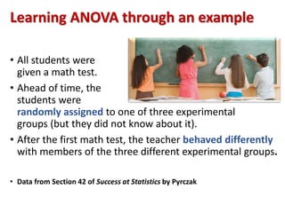
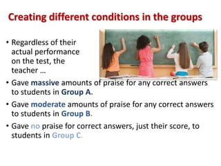
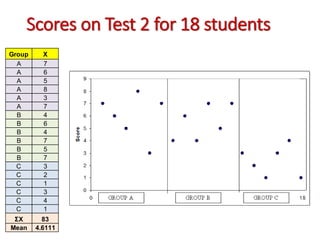
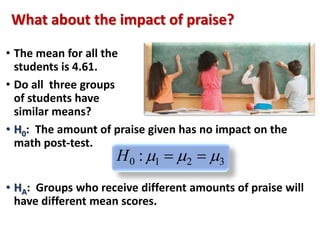
1. Analysis of Variance: Example

2. Learning ANOVA through an example
• All students were
given a math test.
• Ahead of time, the
students were
randomly assigned to one of three experimental
groups (but they did not know about it).
• After the first math test, the teacher behaved differently
with members of the three different experimental groups.
• Data from Section 42 of Success at Statistics by Pyrczak

3. Creating different conditions in the groups
• Regardless of their
actual performance
on the test, the
teacher …
• Gave massive amounts of praise for any correct answers
to students in Group A.
• Gave moderate amounts of praise for any correct answers
to students in Group B.
• Gave no praise for correct answers, just their score, to
students in Group C.

4. Then the variable of interest was
measured
• The next day, at
the end of the math
lesson, the teacher
gave another test.
• Scores for all the students were recorded, as
well as the amount of praise they had received for correct
answers the day before.
• The researchers thought that the earlier praise might
have an effect on their scores on the second test.
• ANOVA’s F-ratio will tell us if that’s true.

5. F test is a ratio of variance BETWEEN groups
and variance WITHIN groups
• On the top: difference between groups, which includes
systematic and random components.
• On the bottom: difference within groups, which includes
only the random component.
• When the systematic component is large, the groups
differ from each other, and F > 1.00
difference s including any treatment effects
difference s with no treatment effects
F 

6. Stating Hypotheses
• H0: The amount of
praise given has
no impact on the
math post-test.
• HA: Groups who receive different amounts of praise
will have different mean scores.

7. Scores on Test 2 for 18 students
Group X
A 7
A 6
A 5
A 8
A 3
A 7
B 4
B 6
B 4
B 7
B 5
B 7
C 3
C 2
C 1
C 3
C 4
C 1
ΣX 83
Mean 4.6111

8. Compare scores to M= 4.61

9. Part II: Variability: distance from the
mean of all the scores on the test

10. Just as in Chapter 3, the differences are squared
Σ(X-M)2 = Sum of Squares = SSTOTAL
Group X Mtotal X-M (X-M)2
A 7 4.6111 2.3889 5.7068
A 6 4.6111 1.3889 1.9290
A 5 4.6111 0.3889 0.1512
A 8 4.6111 3.3889 11.4846
A 3 4.6111 -1.6111 2.5957
A 7 4.6111 2.3889 5.7068
B 4 4.6111 -0.6111 0.3735
B 6 4.6111 1.3889 1.9290
B 4 4.6111 -0.6111 0.3735
B 7 4.6111 2.3889 5.7068
B 5 4.6111 0.3889 0.1512
B 7 4.6111 2.3889 5.7068
C 3 4.6111 -1.6111 2.5957
C 2 4.6111 -2.6111 6.8179
C 1 4.6111 -3.6111 13.0401
C 3 4.6111 -1.6111 2.5957
C 4 4.6111 -0.6111 0.3735
C 1 4.6111 -3.6111 13.0401
Sum of squares: all scores =
SSTOTAL = 80.278
G 83 80.27778 SSTOTAL
Mean 4.6111 4.459877 Variance

11. What about the impact of praise?
• The mean for all the
students is 4.61.
• Do all three groups
of students have
similar means?
• H0: The amount of praise given has no impact on the
math post-test.
0 1 2 3 H :  
• HA: Groups who receive different amounts of praise will
have different mean scores.

12. Compute mean score in the groups
• Mean of Group A: MA=6.00
• Mean of Group B: MB=5.50
• Mean of Group C: MC=2.33
Group X
A 7
A 6
A 5
A 8
A 3
A 7
Mean 6
Group X
B 4
B 6
B 4
B 7
B 5
B 7
Mean 5.5
Group X
C 3
C 2
C 1
C 3
C 4
C 1
Mean 2.333

13. Compare each student’s score to the mean
score for his or her own group
MA=6.00 MB=5.50 MC=2.33

14. Variability within each group is random:
all within group had same amount of praise
SSA=16.00 SSB=9.50 SSC=7.333
Group X MA (X-MA)2
A 7 6 1
A 6 6 0
A 5 6 1
A 8 6 4
A 3 6 9
A 7 6 1
Mean 6 SSA 16.000
Group X MB (X-MB)2
B 4 5.5 2.25
B 6 5.5 0.25
B 4 5.5 2.25
B 7 5.5 2.25
B 5 5.5 0.25
B 7 5.5 2.25
Mean 5.5 SSB 9.500
Group X MC (X-MC)2
C 3 2.333 0.445
C 2 2.333 0.111
C 1 2.333 1.777
C 3 2.333 0.445
C 4 2.333 2.779
C 1 2.333 1.777
Mean 2.333 SSC 7.333

15. Variability within each group is random:
all within group had same amount of praise
To find the amount of
random variability,
add the SS from all
the groups together.
Within Sum of squares
SSwithin=16+9.5+7.33
SSwithin=32.833
SSA=16.00 SSB=9.50 SSC=7.333

16. Part V: Analysis of Variance:
Partitioning variability into components
• SSTOTAL is all the variability in the Sample
• Some of it is systematic variability between groups related to
the treatment, level of praise by the teacher
• Some of it is random within groups, due to the many differences
among students besides the praise level
• SSTOTAL = SSWITHIN + SSBETWEEN

17. Variability between groups is due to the
teacher’s level of praise
• The means of the groups are not the same
• MA=6.00 MB=5.50 MC=2.33
• SSBETWEEN represents the variability due to the different
praise level treatments
• SSTOTAL and SSWITHIN have been computed
• SSTOTAL = 80.28 and SSWITHIN = 32.83
• SSBETWEEN = SSTOTAL – SSWITHIN
• SSBETWEEN = 80.28 – 32.83
• SSBETWEEN = 47.45

18. Part VI: Asking the research question a
new way: as a ratio between variances
• Is the SSBETWEEN large
relative to SSWITHIN ?
• If SSBETWEEN is large
relative to the SSWITHIN
then the treatment (teacher praise) had an effect.
• If SSBETWEEN is large, REJECT the null hypothesis.
• The F-statistic is a ratio of those two components
of variability, adjusted for sample size.
variabilit y including any treatment effects
variabilit y with no treatment effects
F 

19. Compute degrees of freedom
for Sstotal
Sswithin
and SSbetween

20. Each kind of SS has its own df
• Total degrees of freedom for SSTOTAL
dftotal= N – 1 (N is the total number of cases)
dftotal = 18 – 1 = 17
• Between-treatments degrees of freedom for SSBETWEEN
dfbetween= k – 1 (k is the number of groups)
dfbetween= 3 – 1 = 2
• Within-groups degrees of freedom for SSWITHIN
dfwithin= N – k
dfwithin= 18 – 3 = 15

21. “Average” the SSwithin and
SSbetween over their df
These are called
“Mean Squares”

22. Equations for Mean Squares & F
• The between and within sums
of squares are divided by their
df to create the appropriate
variance
• These are called the
Mean Squares
• The SS is averaged (mean)
across df
• The F-ratio test statistic is the
ratio of MSbetween to MSwithin
between
within
SS
SS
within
MS 
MS 
within df
between
between df
between
within
MS
MS
F 

23. Computing the Mean Squares
• SSBETWEEN = 47.45
dfbetween= 3 – 1 = 2
• SSWITHIN = 32.833
dfwithin = 18 – 3 = 15
23.75
47.45
between
SS
  
2
between
between df
MS
2.189
32.833
within
SS
  
15
within
within df
MS

24. Computing F for the example
F = 23.725 / 2.189
10.849 F = 10.849
between
23.735
MS
between
MS
  
2.189
within
MS
F
within
MS
F 

25. Testing hypotheses with F
10.849
23.75
between
MS
  
2.189
within
MS
F
• When the p-value for F is less than the alpha you chose
for your test, then you can Reject H0
• There are critical values for F that define a rejection region
– but they vary by both types of df and (outside of intro
statistics courses) no one knows any of them by heart.
• In this class: we use p-value only, from the F Distribution
calculator.

26. Testing hypotheses with F
10.849
23.75
between
MS
  
2.189
within
MS
F
• The p-value of F = 10.849 for df = 2, 15 is p=.0012
• Using  = .05
• Since the p-value is less than (<) the alpha level, we
Reject the null hypothesis.
• Some groups had different levels of performance on the
test due to the level of the teacher’s praise.

27. ANOVA table – a tool for computing F
Source SS df MS F
Between 47.45 2 23.725 10.84
Within 32.83 15 2.189
Total 80.28 17
• The SS and df columns add up to the total
• In each row, SS divided by df equals MS
• In the final column, F is MSB divided by MSW

28. 1. Fill in the blanks.
2. How many subjects were in the study?
3. How many groups were in the study?

29. Review of the ANOVA test
• Hypotheses and significance level are stated
• Sum of Squared differences from the mean of all the
scores is computed = SStotal
• Sum of Squared differences from the mean of each group
is computed = SSwithin
• Sum of Squared differences between groups is computed
by subtraction = SSbetween
• Degrees of Freedom df are computed for each SS
• Mean Squares MSbetween and MSwithin are computed.
• F ratio is computed and its p –value determined.
• Decision is made regarding the null hypothesis.