Downloaded 668 times


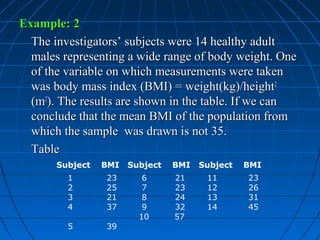


BMI (kg/m2) 22.1 23.4 24.8 26.2 27.6 28.9 30.3 31.6 32.9 34.2 35.5 36.8 38.1 39.4 The sample mean is 29.1 kg/m2 and the sample standard deviation is 4.2 kg/m2. Test the hypothesis that the population mean BMI is 30 kg/m2 at 5% level of significance.