Bisection method

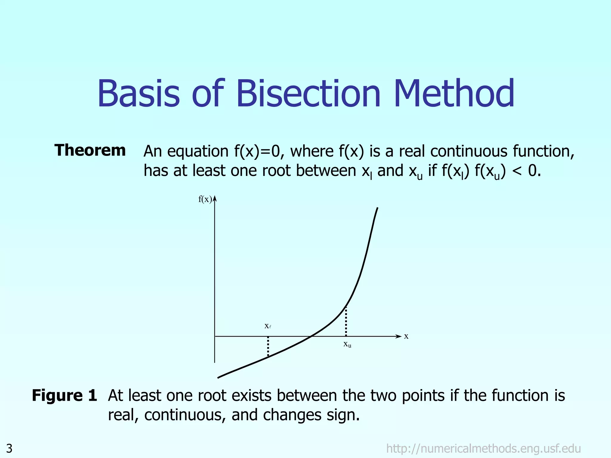
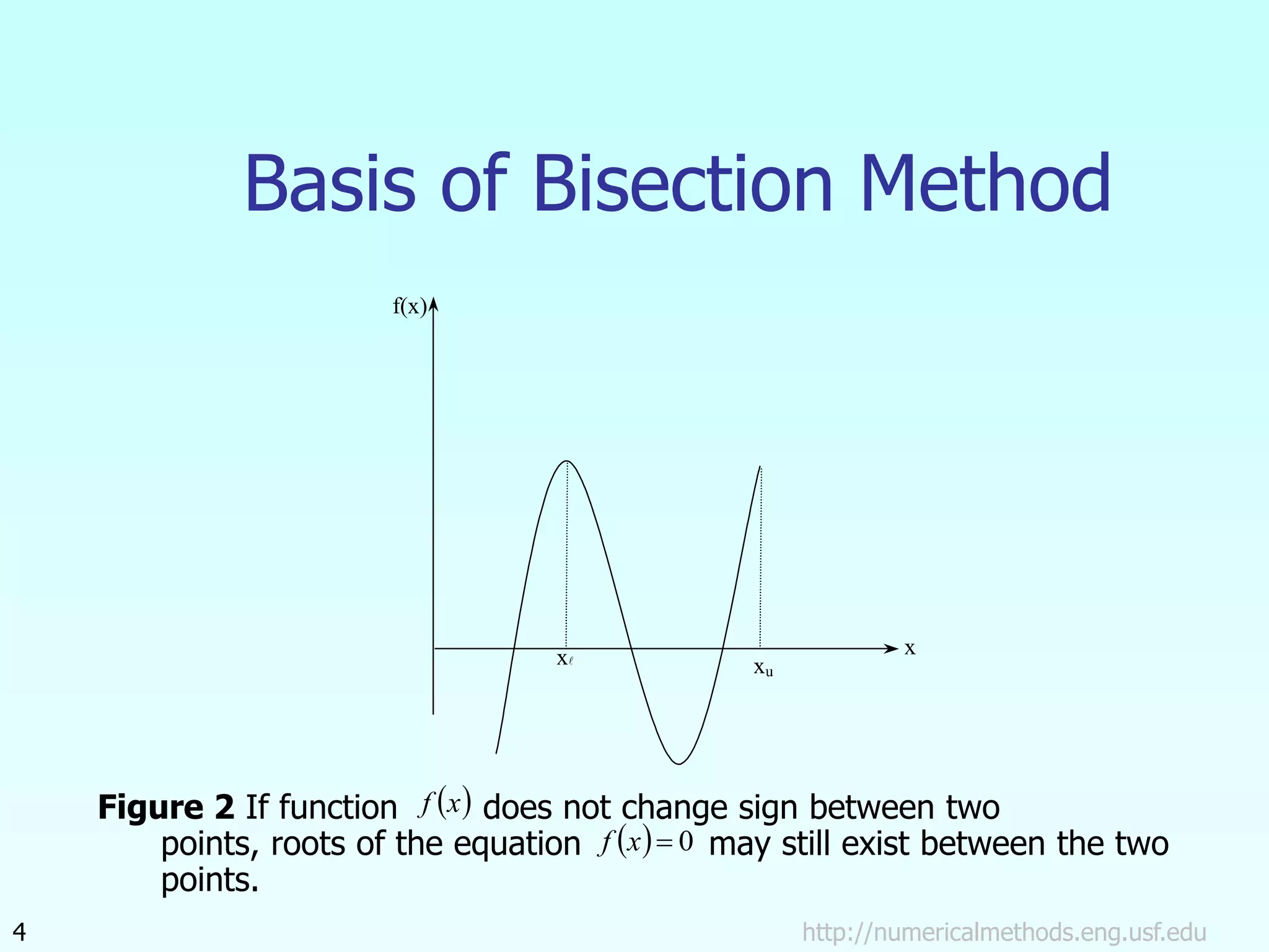
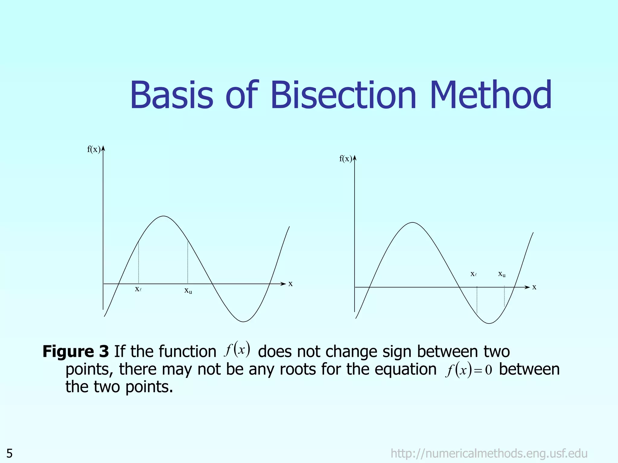
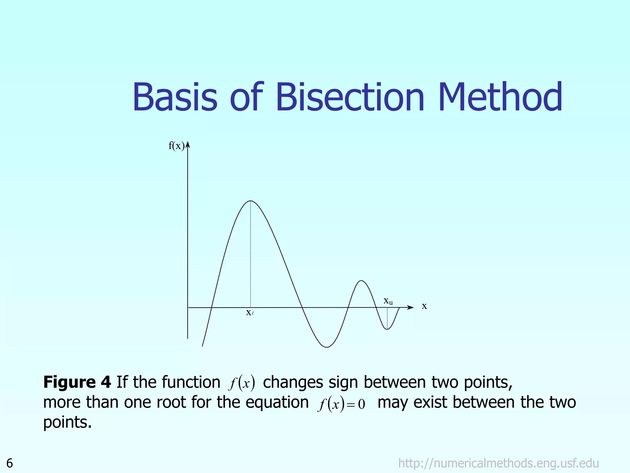
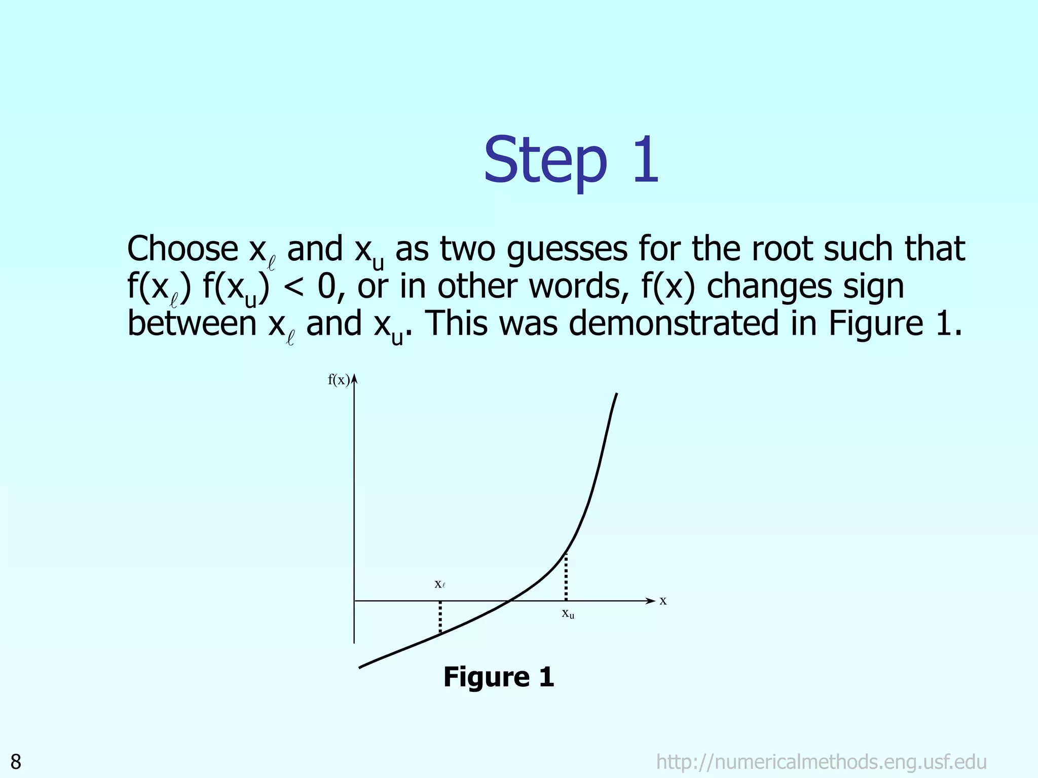
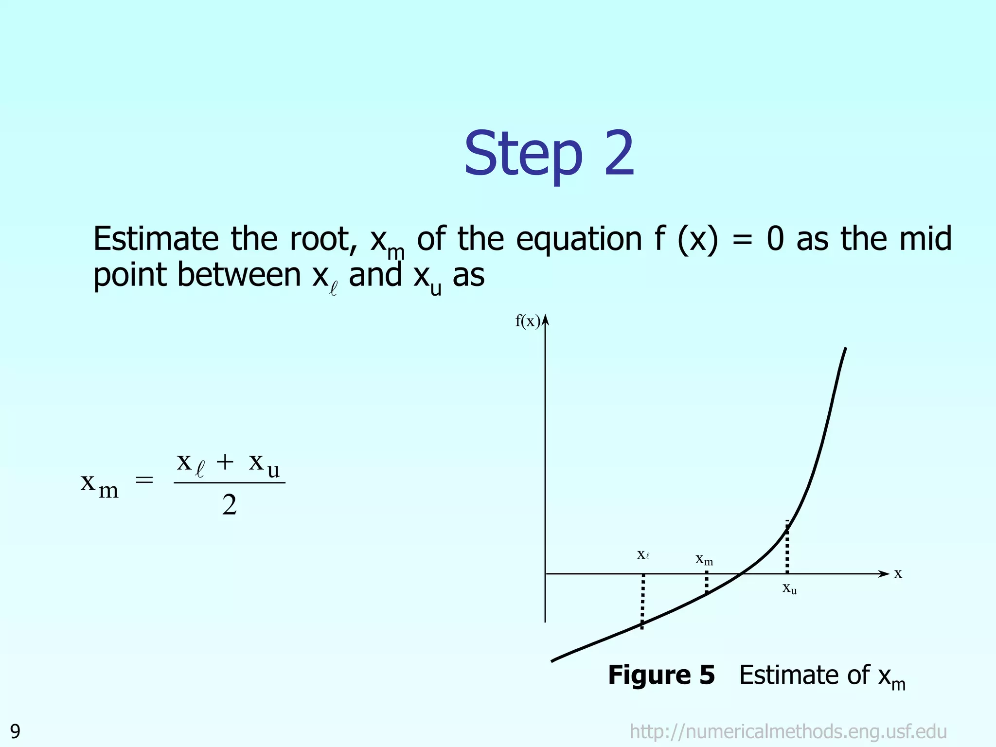
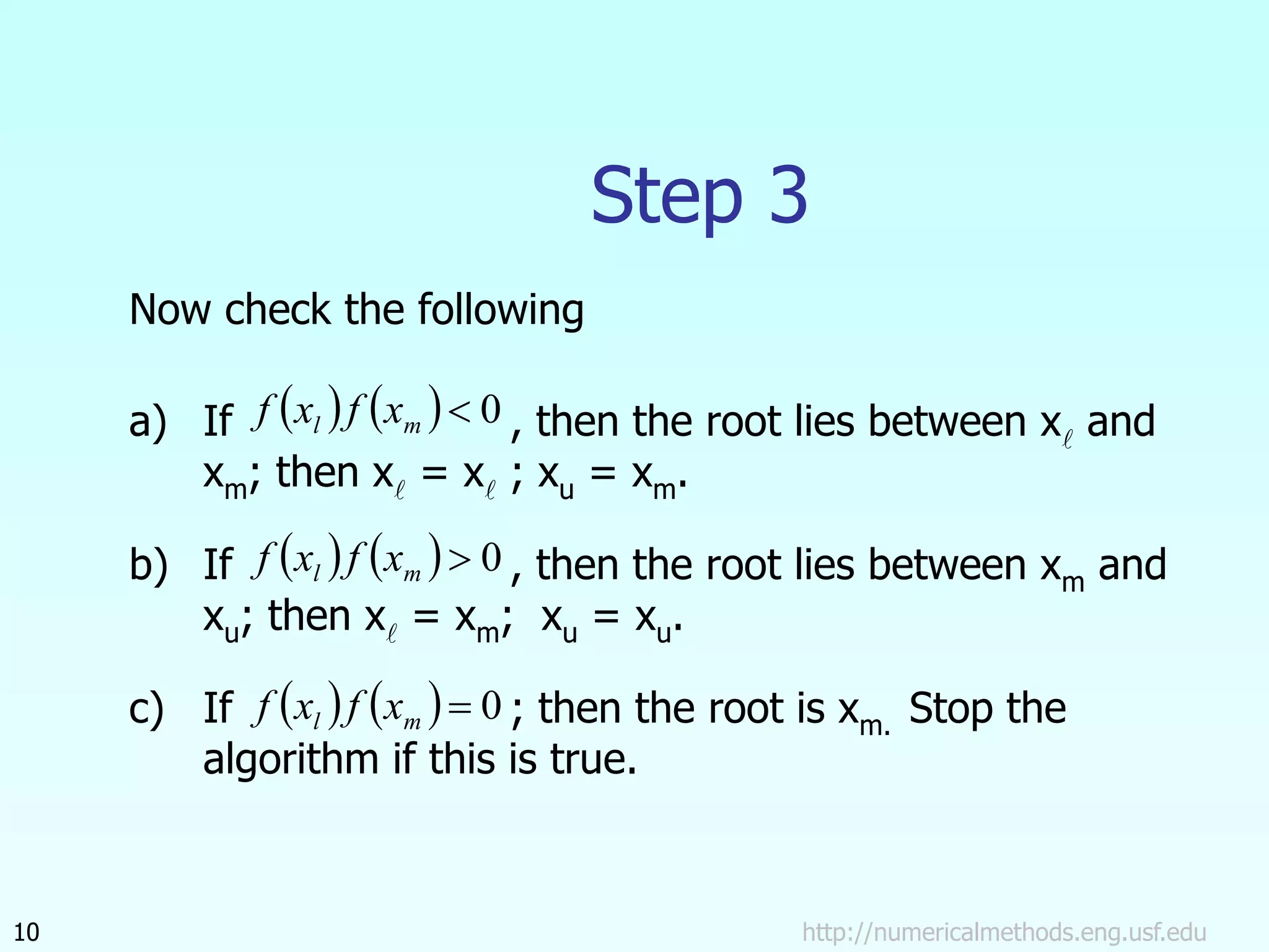
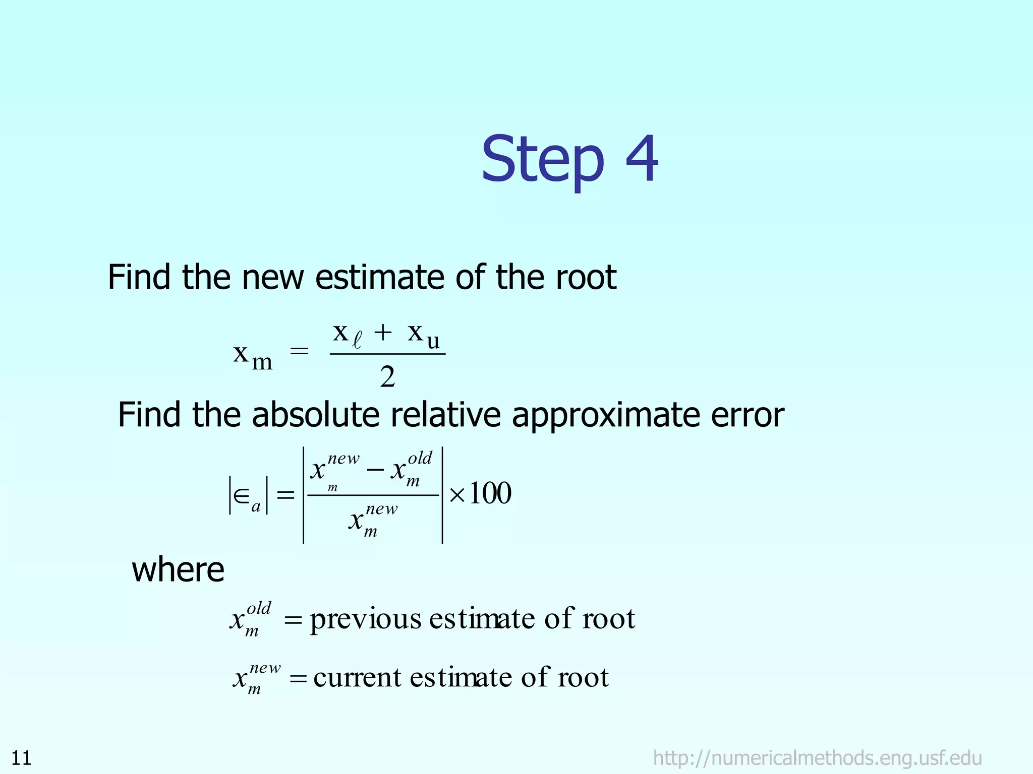
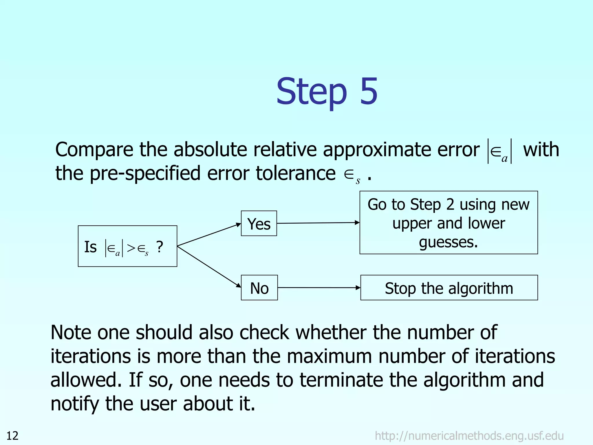
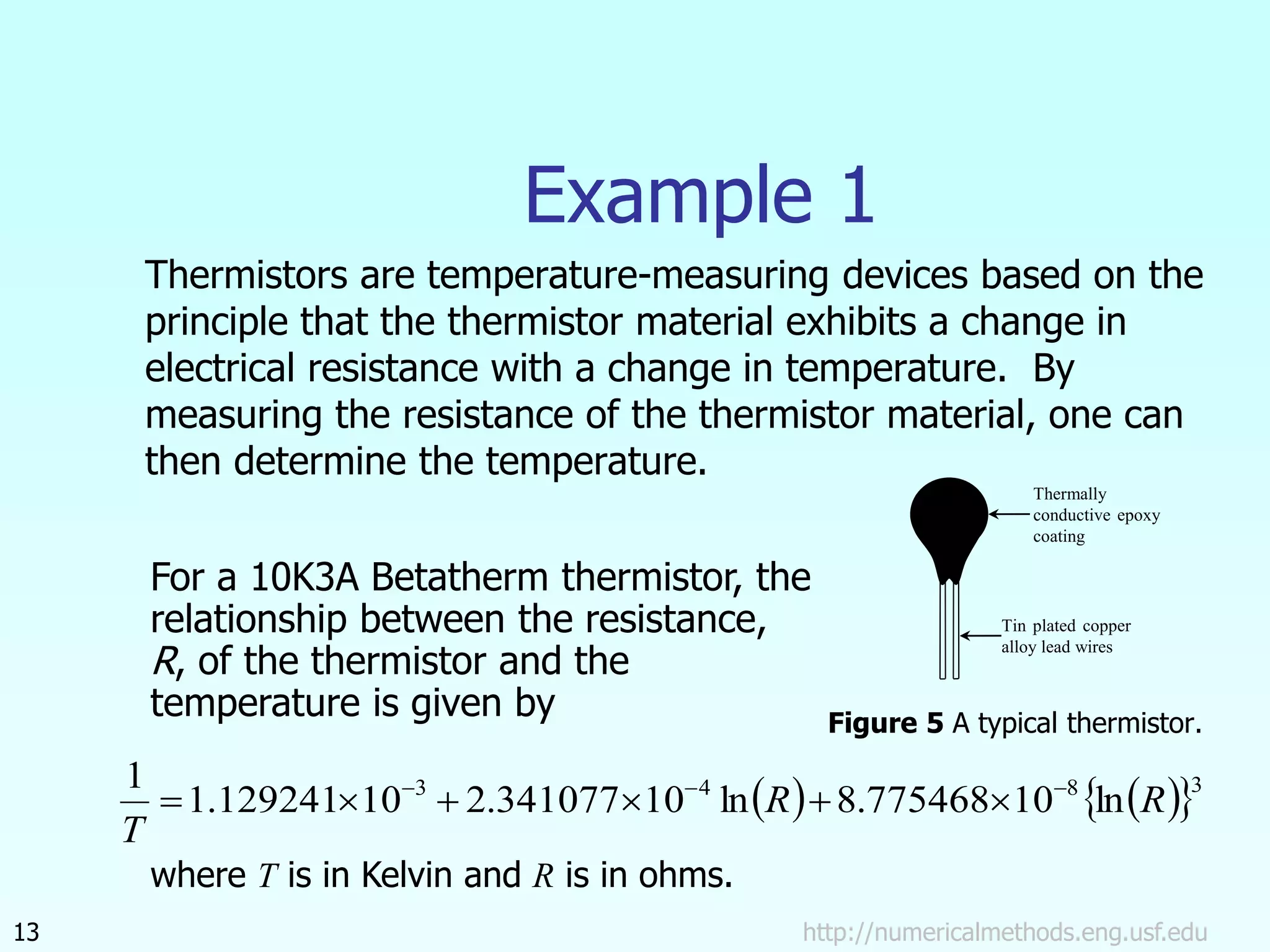
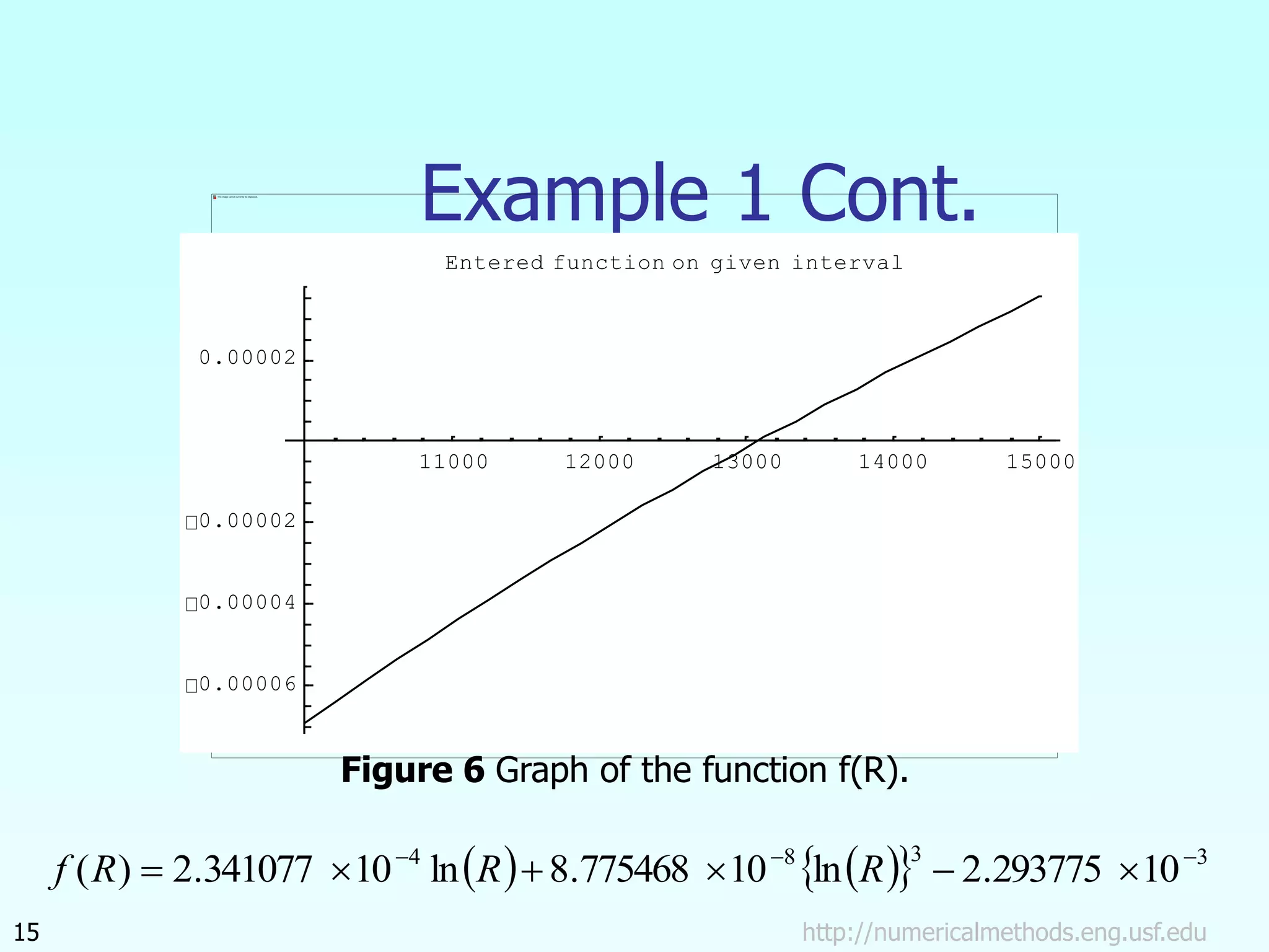
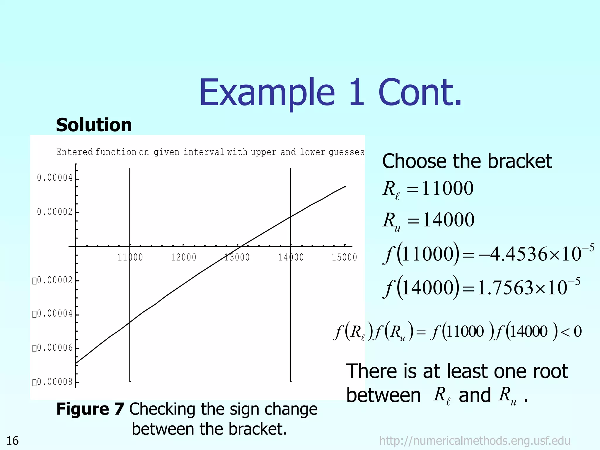
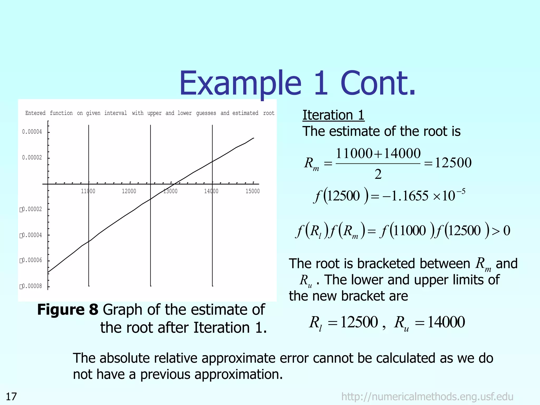
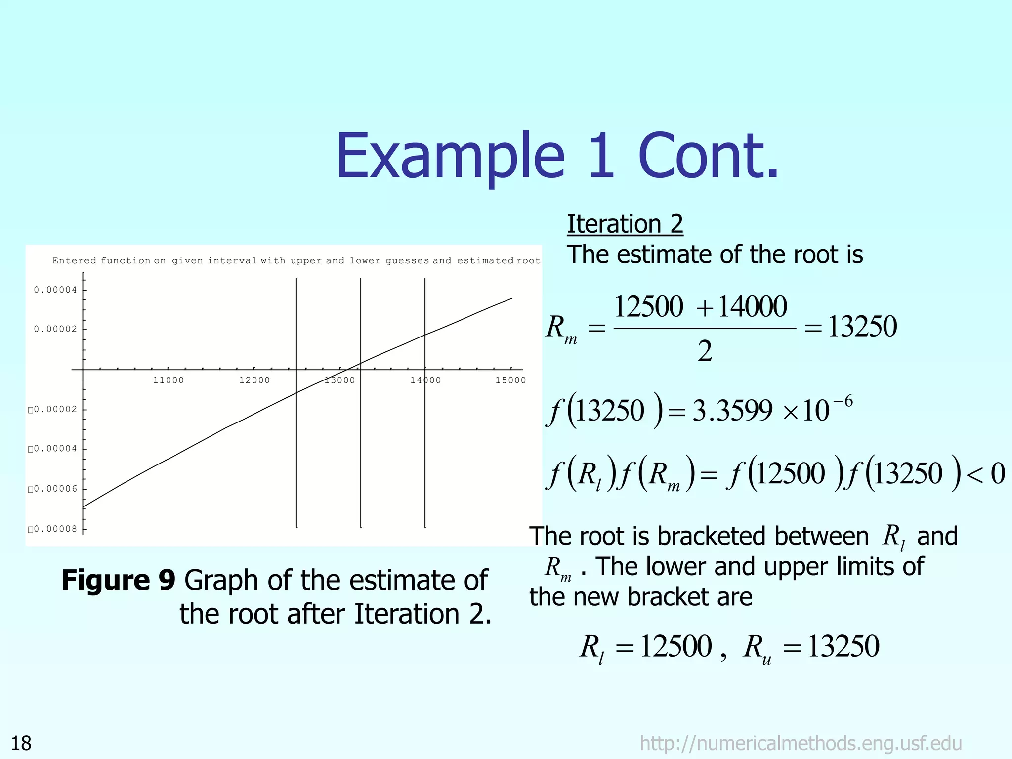
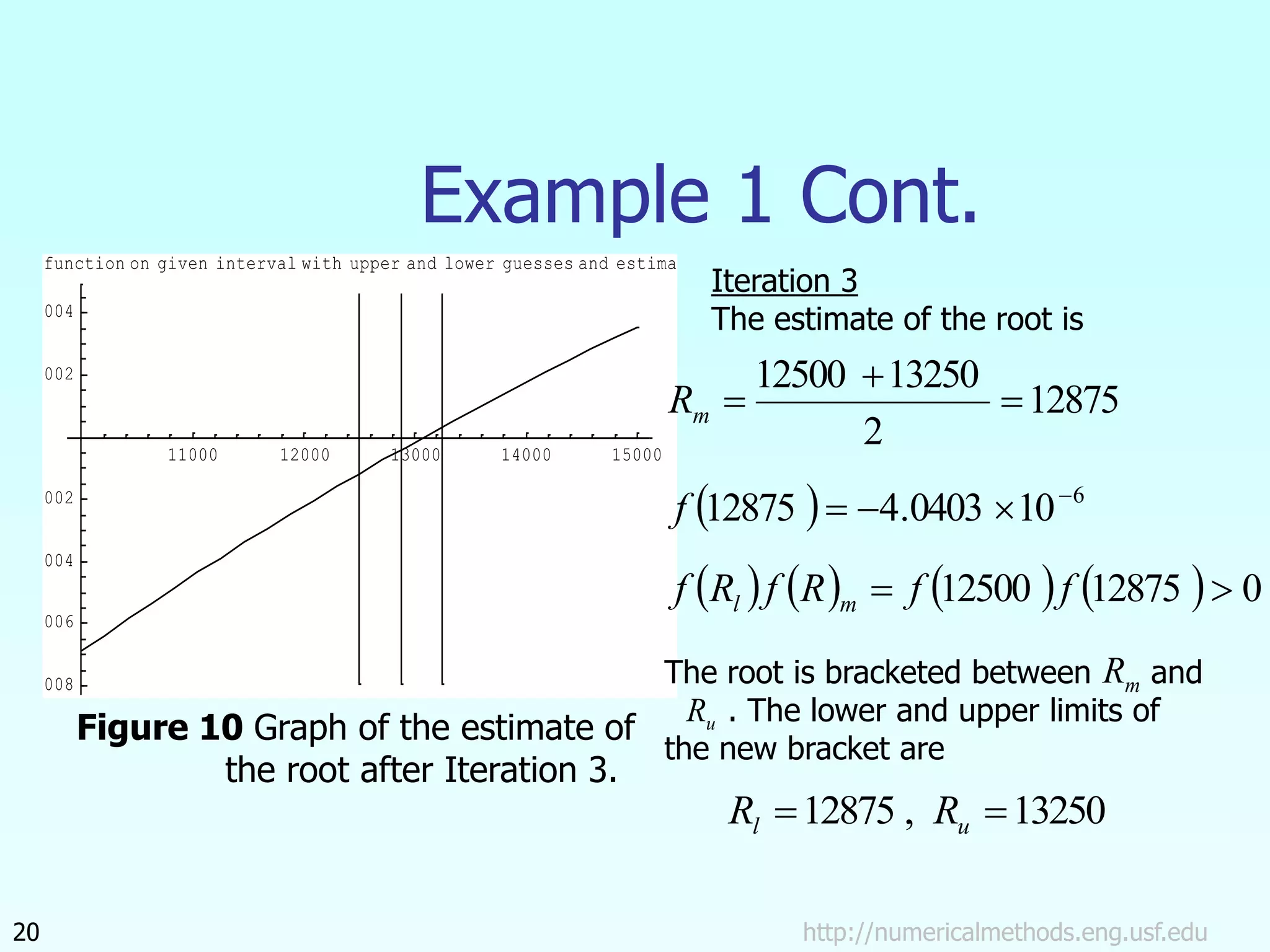
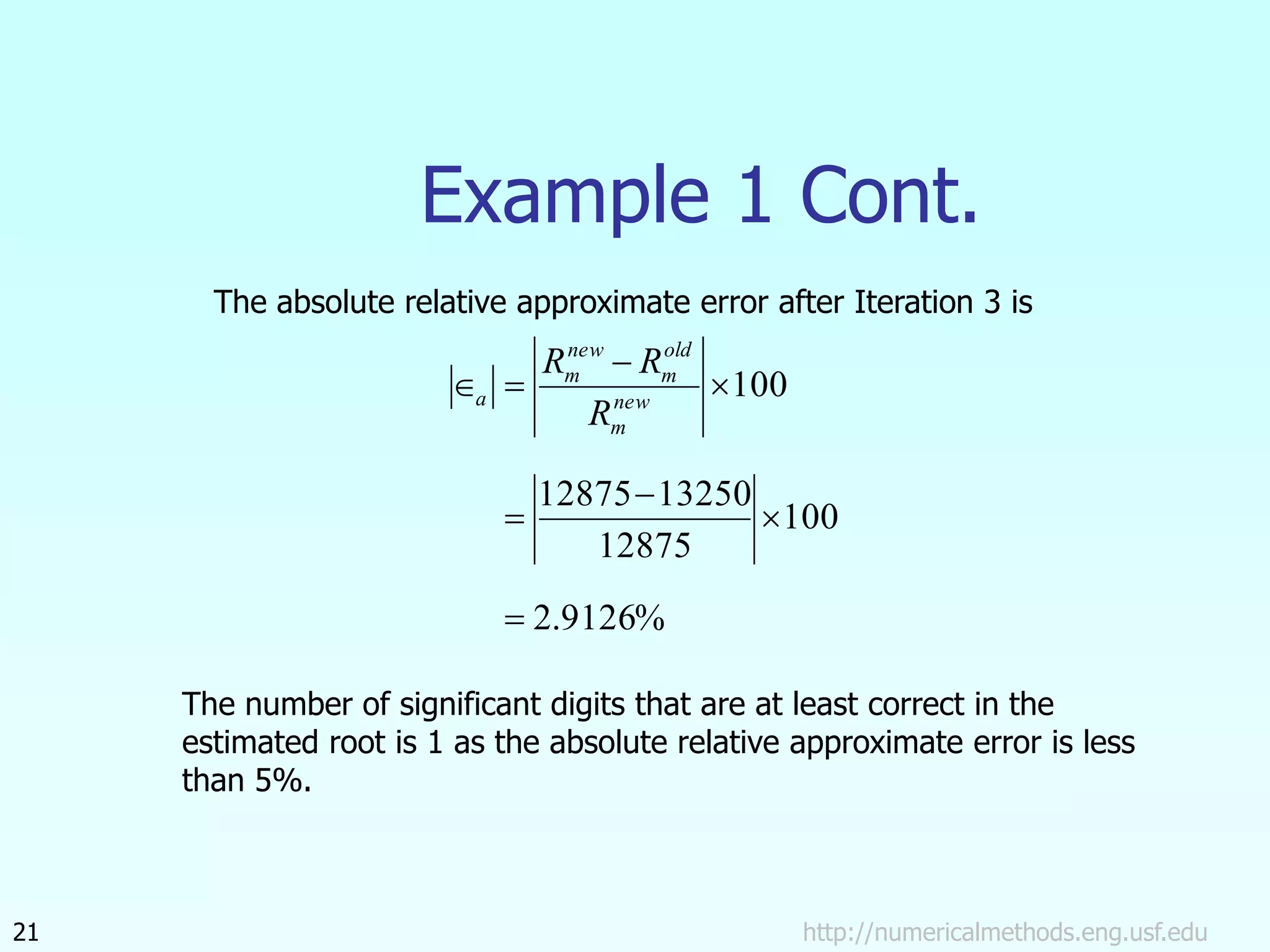
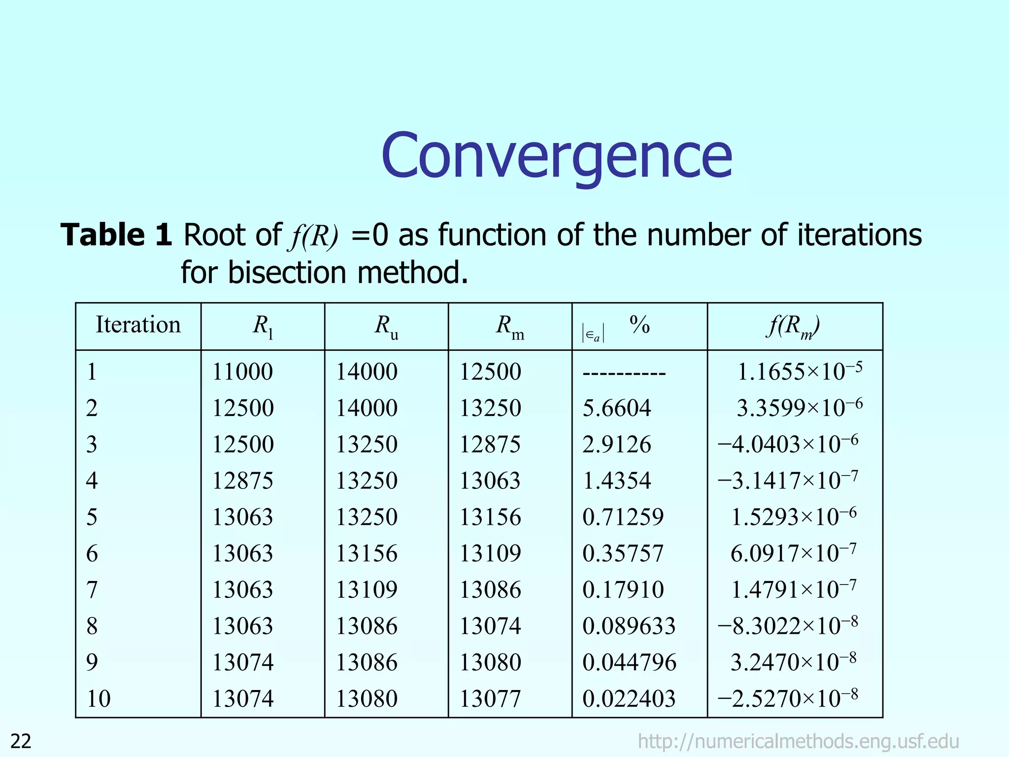
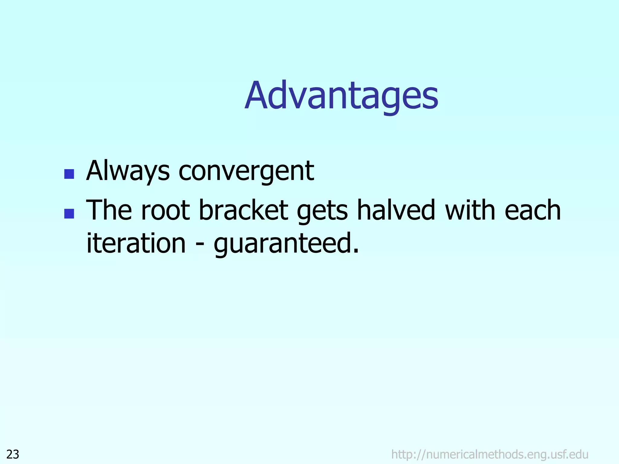
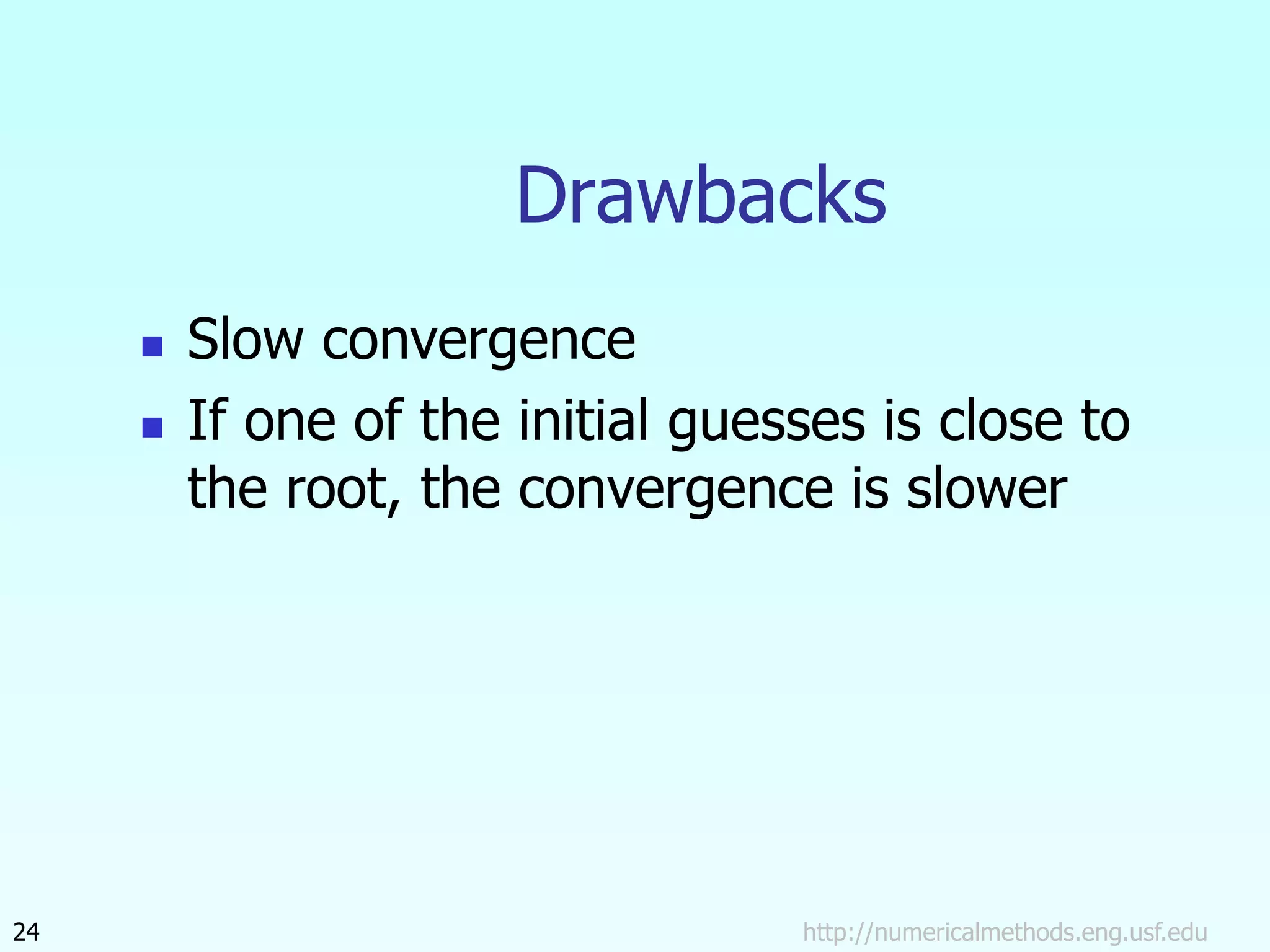
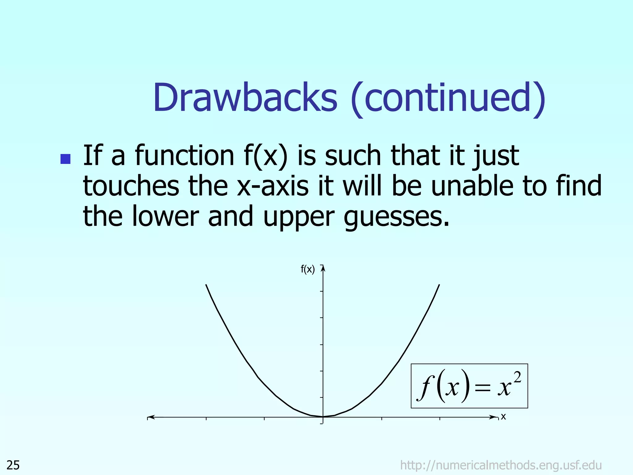
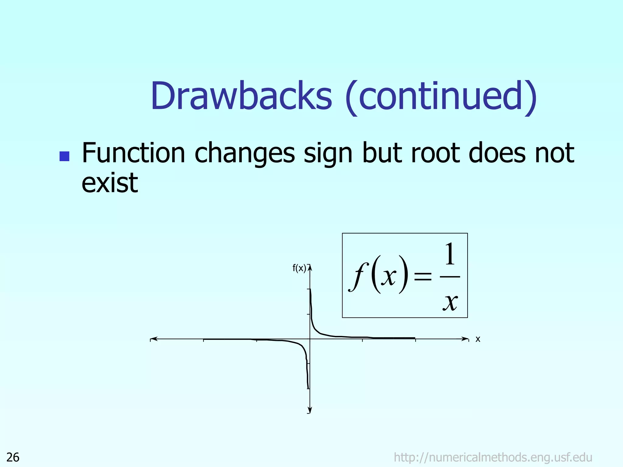
8/17/2022 http://numericalmethods.eng.usf.edu 1
Bisection Method
Electrical Engineering Majors
Authors: Autar Kaw, Jai Paul
http://numericalmethods.eng.usf.edu
Transforming Numerical Methods Education for STEM
Undergraduates

Bisection Method

3
Basis of Bisection Method
Theorem
x
f(x)
xu
x
An equation f(x)=0, where f(x) is a real continuous function,
has at least one root between xl and xu if f(xl) f(xu) < 0.
Figure 1 At least one root exists between the two points if the function is
real, continuous, and changes sign.

x
f(x)
xu
x
4
Figure 2 If function does not change sign between two
points, roots of the equation may still exist between the two
points.
 
x
f
  0

x
f

x
f(x)
xu
x
5
Figure 3 If the function does not change sign between two
points, there may not be any roots for the equation between
the two points.
x
f(x)
xu
x
 
x
f
  0

x
f

x
f(x)
xu
x
6
Figure 4 If the function changes sign between two points,
more than one root for the equation may exist between the two
points.
 
x
f
  0

x
f

7
Algorithm for Bisection Method

8
Step 1
Choose x and xu as two guesses for the root such that
f(x) f(xu) < 0, or in other words, f(x) changes sign
between x and xu. This was demonstrated in Figure 1.
x
f(x)
xu
x
Figure 1

x
f(x)
xu
x
xm
9
Step 2
Estimate the root, xm of the equation f (x) = 0 as the mid
point between x and xu as
x
x
m =
xu
 
2
Figure 5 Estimate of xm

10
Step 3
Now check the following
a) If , then the root lies between x and
xm; then x = x ; xu = xm.
b) If , then the root lies between xm and
xu; then x = xm; xu = xu.
c) If ; then the root is xm. Stop the
algorithm if this is true.
    0

m
l x
f
x
f
    0

m
l x
f
x
f
    0

m
l x
f
x
f

11
Step 4
x
x
m =
xu
 
2
100



 new
m
old
m
new
a
x
x
xm
root
of
estimate
current

new
m
x
root
of
estimate
previous

old
m
x
Find the new estimate of the root
Find the absolute relative approximate error
where

12
Step 5
Is ?
Yes
No
Go to Step 2 using new
upper and lower
guesses.
Stop the algorithm
Compare the absolute relative approximate error with
the pre-specified error tolerance .
a

s

s
a 

Note one should also check whether the number of
iterations is more than the maximum number of iterations
allowed. If so, one needs to terminate the algorithm and
notify the user about it.

   
 3
8
4
3
ln
10
775468
.
8
ln
10
341077
.
2
10
129241
.
1
1
R
R
T









13
Example 1
Thermistors are temperature-measuring devices based on the
principle that the thermistor material exhibits a change in
electrical resistance with a change in temperature. By
measuring the resistance of the thermistor material, one can
then determine the temperature.
Figure 5 A typical thermistor.
For a 10K3A Betatherm thermistor, the
relationship between the resistance,
R, of the thermistor and the
temperature is given by
where T is in Kelvin and R is in ohms.
Thermally
conductive epoxy
coating
Tin plated copper
alloy lead wires

14
Example 1 Cont.
For the thermistor, error of no more than ±0.01oC is acceptable.
To find the range of the resistance that is within this acceptable
limit at 19oC, we need to solve
and
Use the bisection method of finding roots of equations to find the
resistance R at 18.99oC.
a) Conduct three iterations to estimate the root of the above
equation.
b) Find the absolute relative approximate error at the end of each
iteration and the number of significant digits at least correct at
the end of each iteration.
   
 3
8
4
3
ln
10
775468
.
8
ln
10
341077
.
2
10
129241
.
1
15
.
273
01
.
19
1
R
R 









   
 3
8
4
3
ln
10
775468
.
8
ln
10
341077
.
2
10
129241
.
1
15
.
273
99
.
18
1
R
R 










15
Example 1 Cont.
   
  3
3
8
4
10
293775
.
2
ln
10
775468
.
8
ln
10
341077
.
2
)
( 







 R
R
R
f
11000 12000 13000 14000 15000
0.00006
0.00004
0.00002
0.00002
Entered function on given interval
Figure 6 Graph of the function f(R).

16
Example 1 Cont.
Choose the bracket
 
  5
5
10
7563
.
1
14000
10
4536
.
4
11000
14000
11000









f
f
R
R
u

11000 12000 13000 14000 15000
0.00008
0.00006
0.00004
0.00002
0.00002
0.00004
Entered function on given interval with upper and lower guesses
Solution
        0
14000
11000 
 f
f
R
f
R
f u

There is at least one root
between and .

R u
R
Figure 7 Checking the sign change
between the bracket.

The absolute relative approximate error cannot be calculated as we do
not have a previous approximation.
17
12500
2
14000
11000



m
R
  5
10
1655
.
1
12500 



f
11000 12000 13000 14000 15000
0.00008
0.00006
0.00004
0.00002
0.00002
0.00004
Entered function on given interval with upper and lower guesses and estimated root
Example 1 Cont.
Iteration 1
The estimate of the root is
Figure 8 Graph of the estimate of
the root after Iteration 1.
The root is bracketed between and
. The lower and upper limits of
the new bracket are
14000
,
12500 
 u
l R
R
u
R
m
R
        0
12500
11000 
 f
f
R
f
R
f m
l

11000 12000 13000 14000 15000
0.00008
0.00006
0.00004
0.00002
0.00002
0.00004
Entered function on given interval with upper and lower guesses and estimated root
the new bracket are
Example 1 Cont.
18
 
        0
13250
12500
10
3599
.
3
13250
13250
2
14000
12500
6








f
f
R
f
R
f
f
R
m
l
m
Iteration 2
13250
,
12500 
 u
l R
R
m
R
l
R

Example 1 Cont.
19
%
6604
.
5
100
13250
12500
13250
100







 new
m
old
m
new
m
a
R
R
R
The absolute relative approximate error after Iteration 2 is
None of the significant digits are at least correct in the estimated root
as the absolute relative approximate error is greater than 5%.

11000 12000 13000 14000 15000
0.00008
0.00006
0.00004
0.00002
0.00002
0.00004
ered function on given interval with upper and lower guesses and estimated root
20
 
        0
12875
12500
10
0403
.
4
12875
12875
2
13250
12500
6









f
f
R
f
R
f
f
R
m
l
m
the new bracket are
Iteration 3
13250
,
12875 
 u
l R
R
u
R
m
R
Example 1 Cont.

Example 1 Cont.
21
%
9126
.
2
100
12875
13250
12875
100







 new
m
old
m
new
m
a
R
R
R
The absolute relative approximate error after Iteration 3 is
The number of significant digits that are at least correct in the
estimated root is 1 as the absolute relative approximate error is less
than 5%.

22
Convergence
Table 1 Root of f(R) =0 as function of the number of iterations
for bisection method.
a
Iteration Rl Ru Rm % f(Rm)
1
2
3
4
5
6
7
8
9
10
11000
12500
12500
12875
13063
13063
13063
13063
13074
13074
14000
14000
13250
13250
13250
13156
13109
13086
13086
13080
12500
13250
12875
13063
13156
13109
13086
13074
13080
13077
----------
5.6604
2.9126
1.4354
0.71259
0.35757
0.17910
0.089633
0.044796
0.022403
1.1655×10−5
3.3599×10−6
−4.0403×10−6
−3.1417×10−7
1.5293×10−6
6.0917×10−7
1.4791×10−7
−8.3022×10−8
3.2470×10−8
−2.5270×10−8

23
Advantages
 Always convergent
 The root bracket gets halved with each
iteration - guaranteed.

24
Drawbacks
 Slow convergence
 If one of the initial guesses is close to
the root, the convergence is slower

25
Drawbacks (continued)
 If a function f(x) is such that it just
touches the x-axis it will be unable to find
the lower and upper guesses.
f(x)
x
  2
x
x
f 

26
Drawbacks (continued)
 Function changes sign but root does not
exist
f(x)
x
 
x
x
f
1


Additional Resources
For all resources on this topic such as digital audiovisual
lectures, primers, textbook chapters, multiple-choice
tests, worksheets in MATLAB, MATHEMATICA, MathCad
and MAPLE, blogs, related physical problems, please
visit
http://numericalmethods.eng.usf.edu/topics/bisection_
method.html

THE END

Bisection method

More Related Content

What's hot

Similar to Bisection method

Recently uploaded

Bisection method