The document describes the bisection method for finding the root of an equation. It begins by establishing the basis of the bisection method, which is that if a continuous function changes sign between two points, there is at least one root between those points. It then provides the step-by-step algorithm for implementing the bisection method to iteratively find the root. Finally, it includes an example of applying the bisection method to find the depth at which a floating ball is submerged.

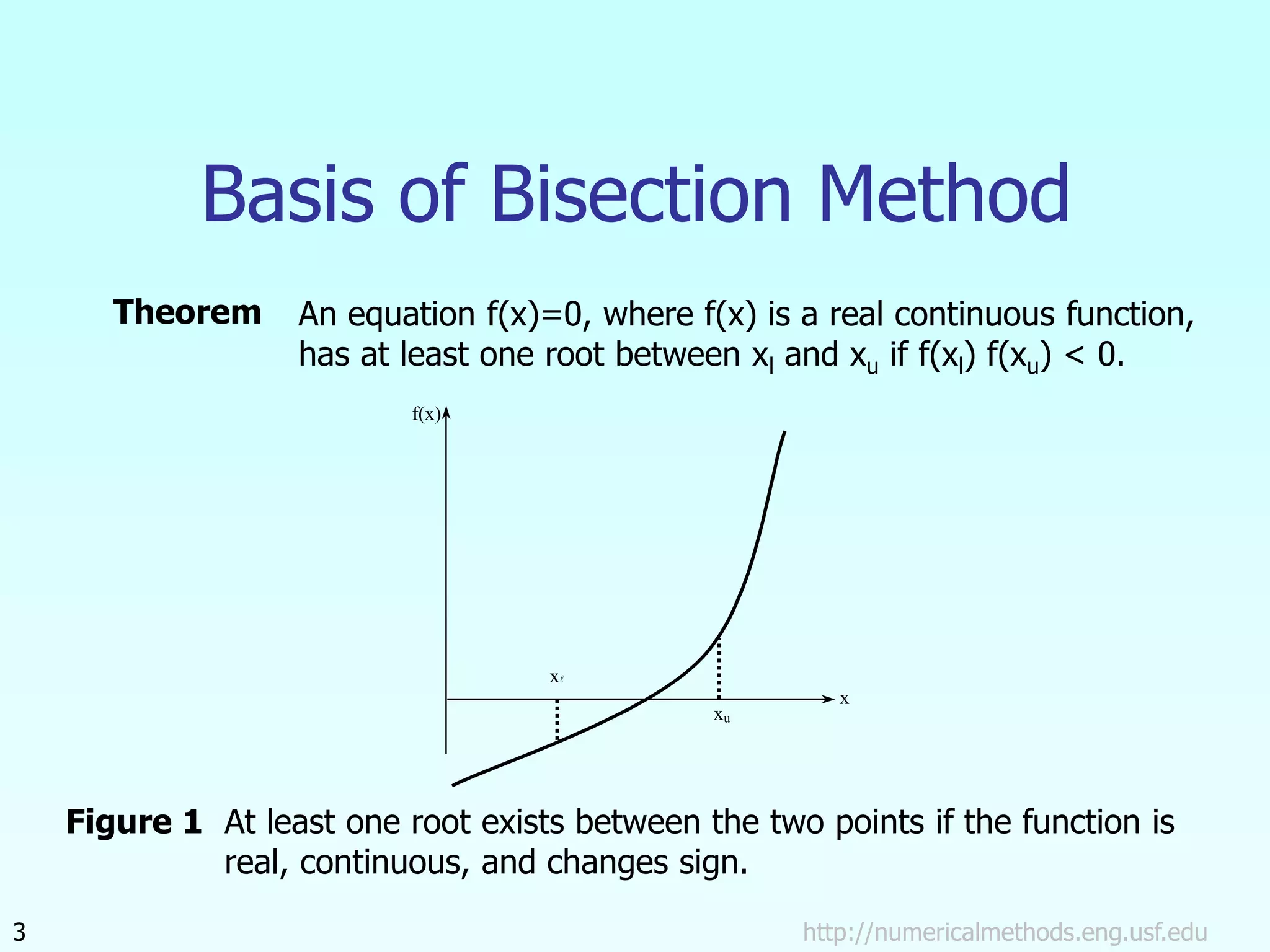
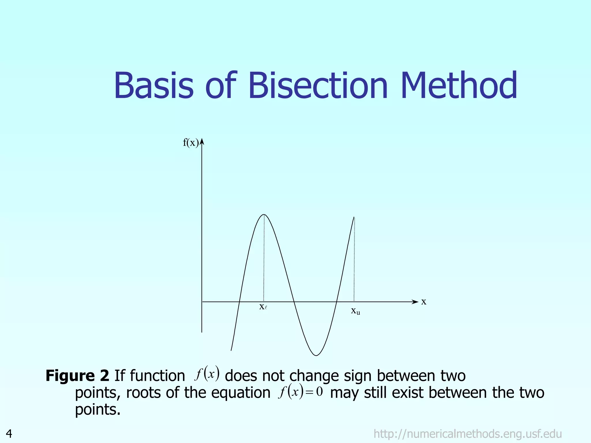
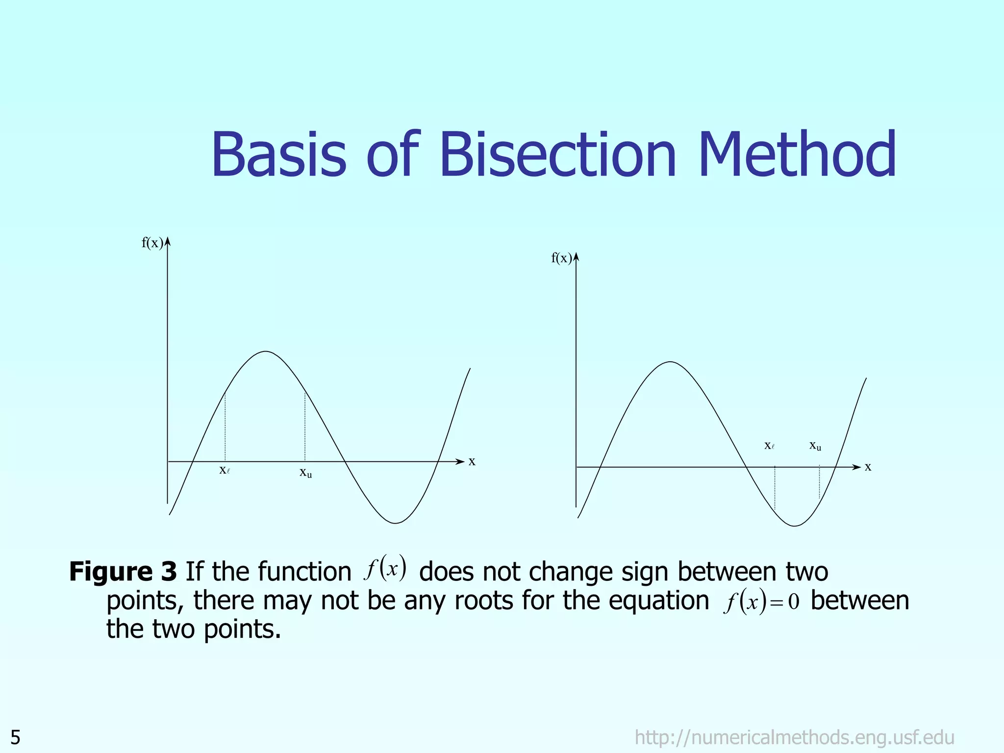
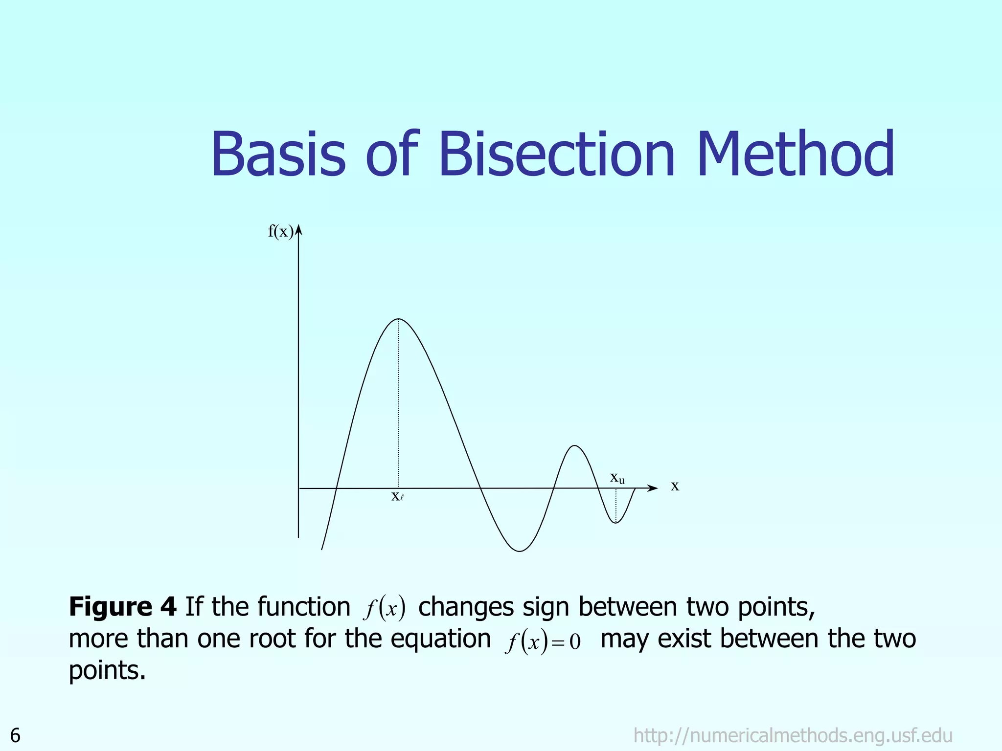
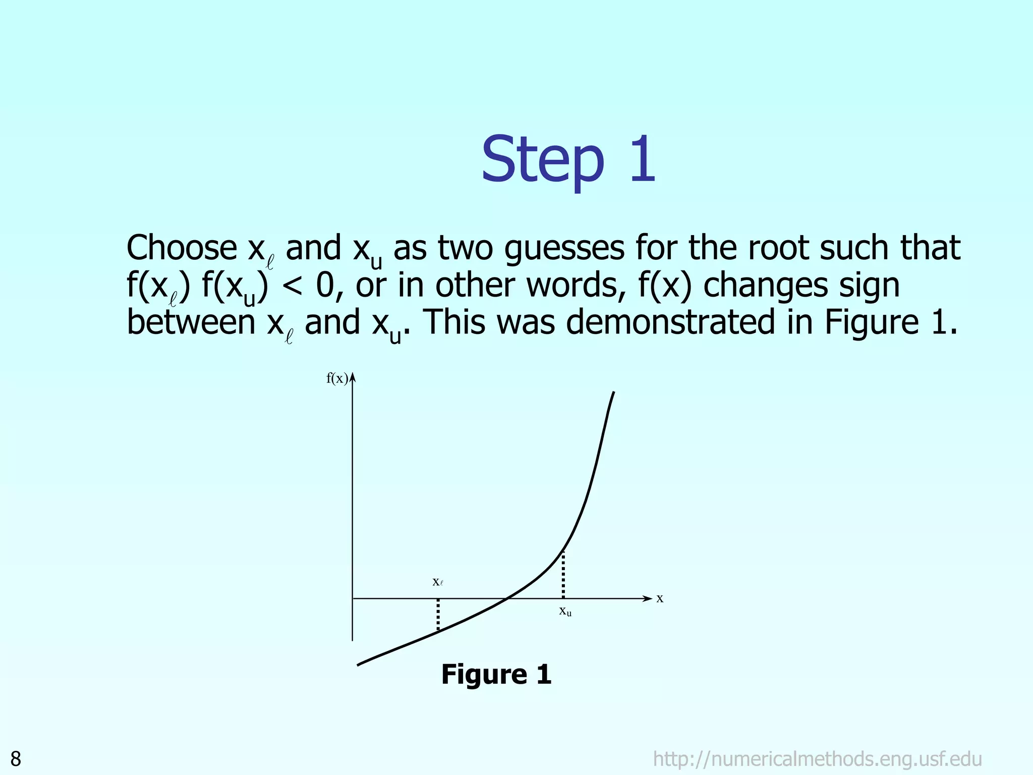
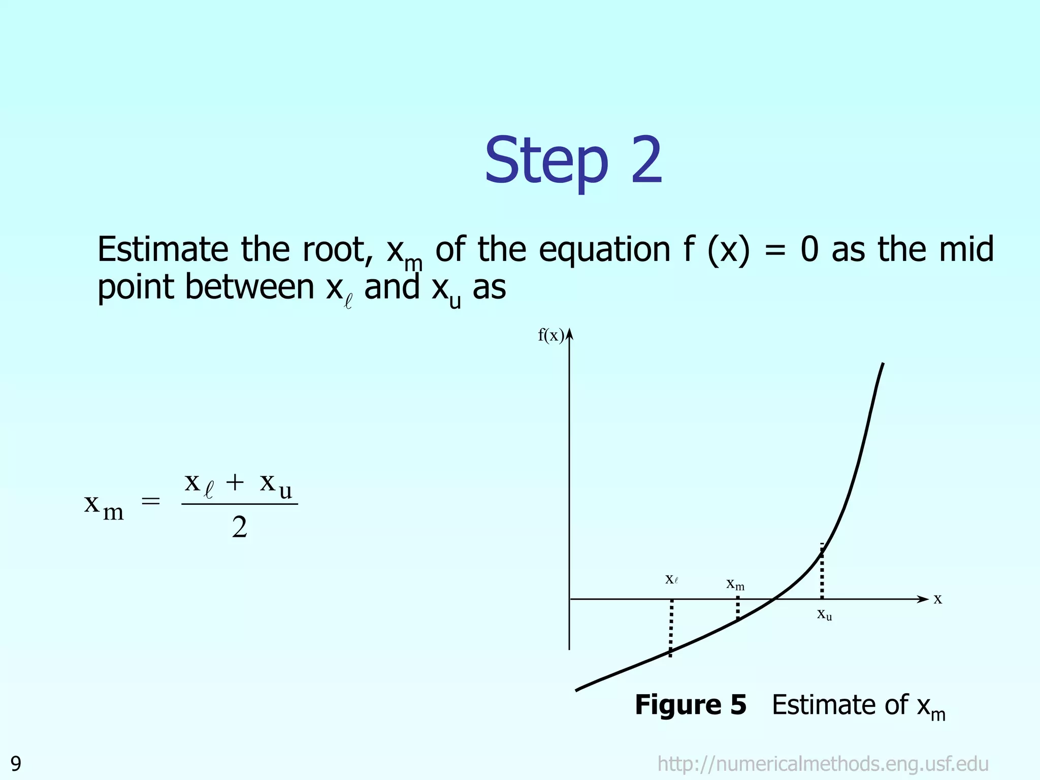
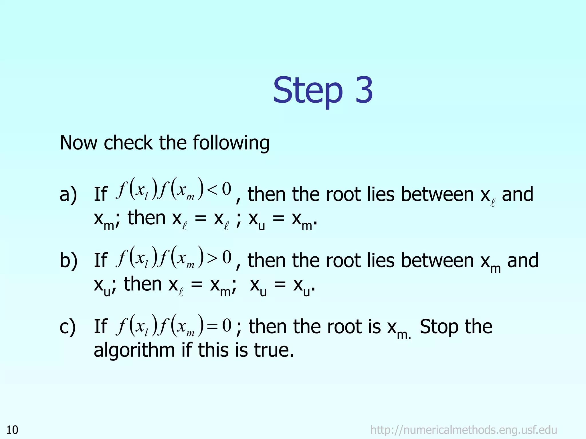
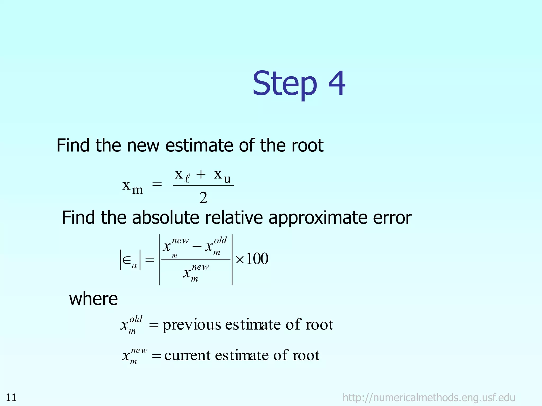
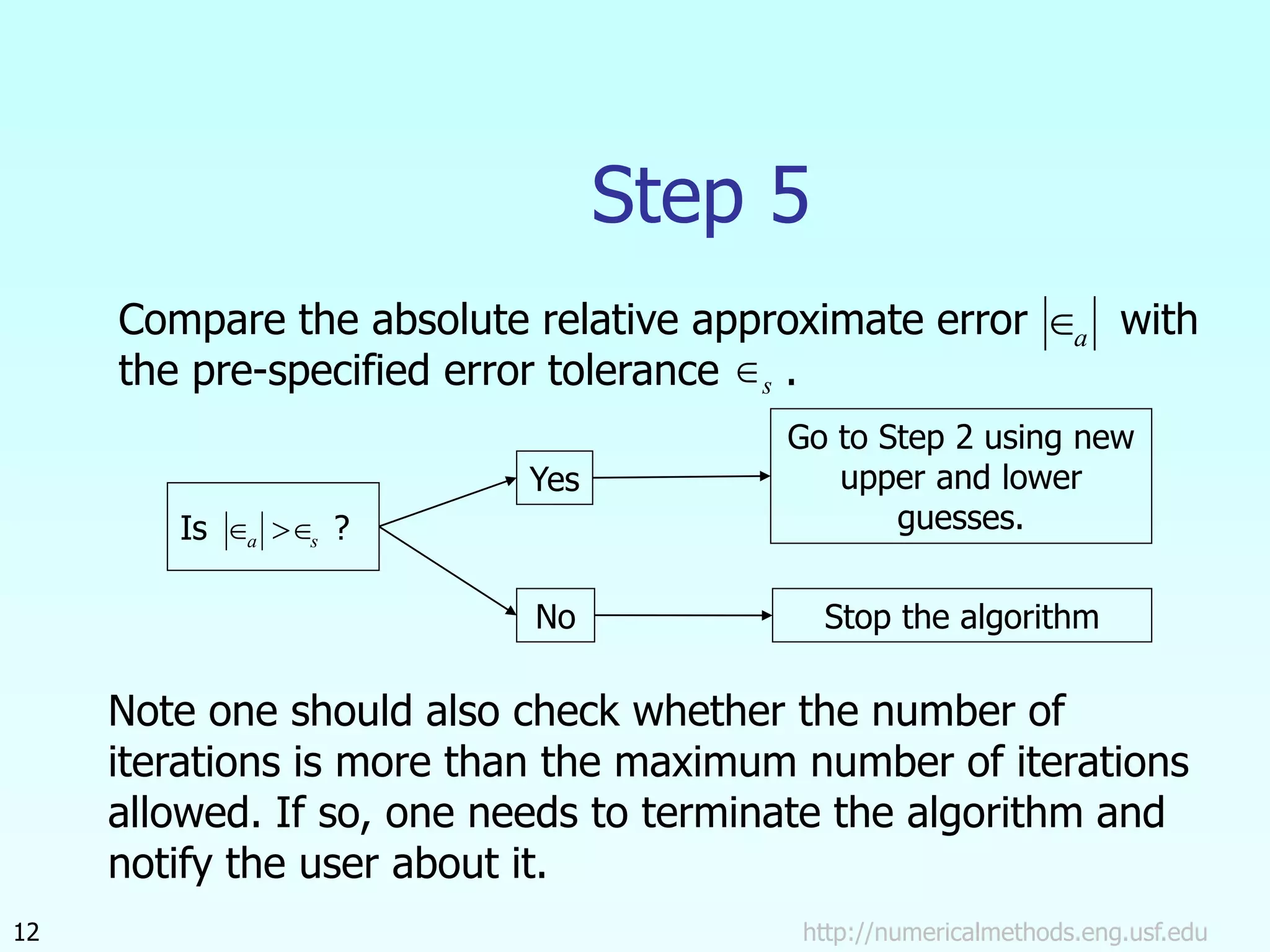
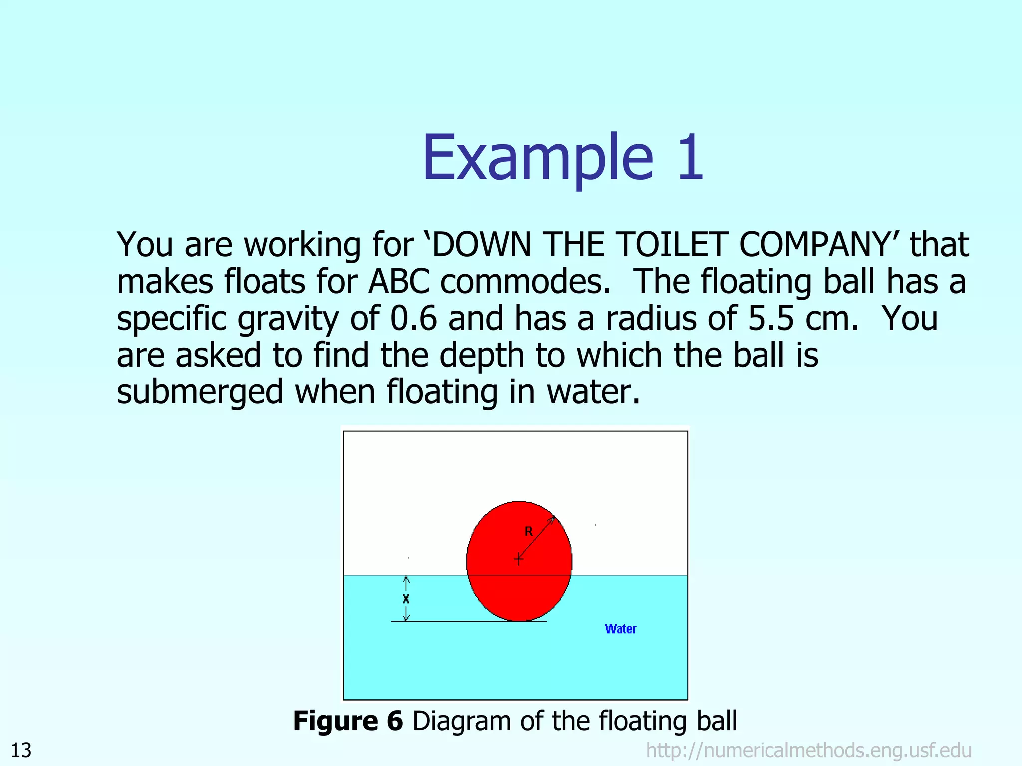
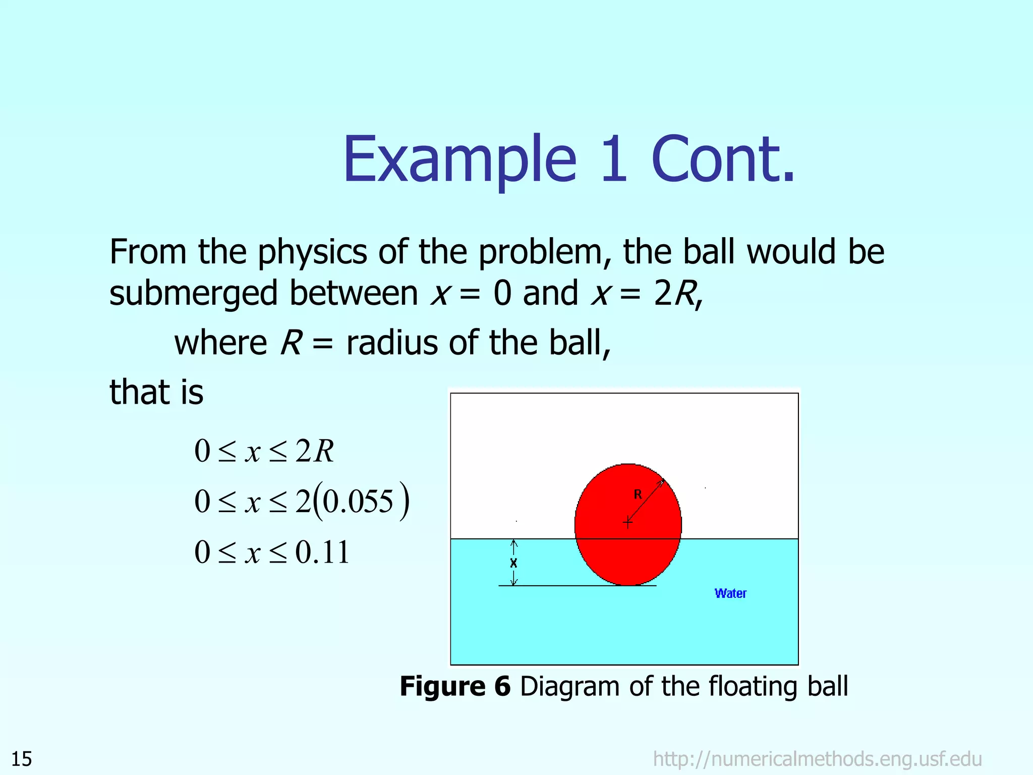
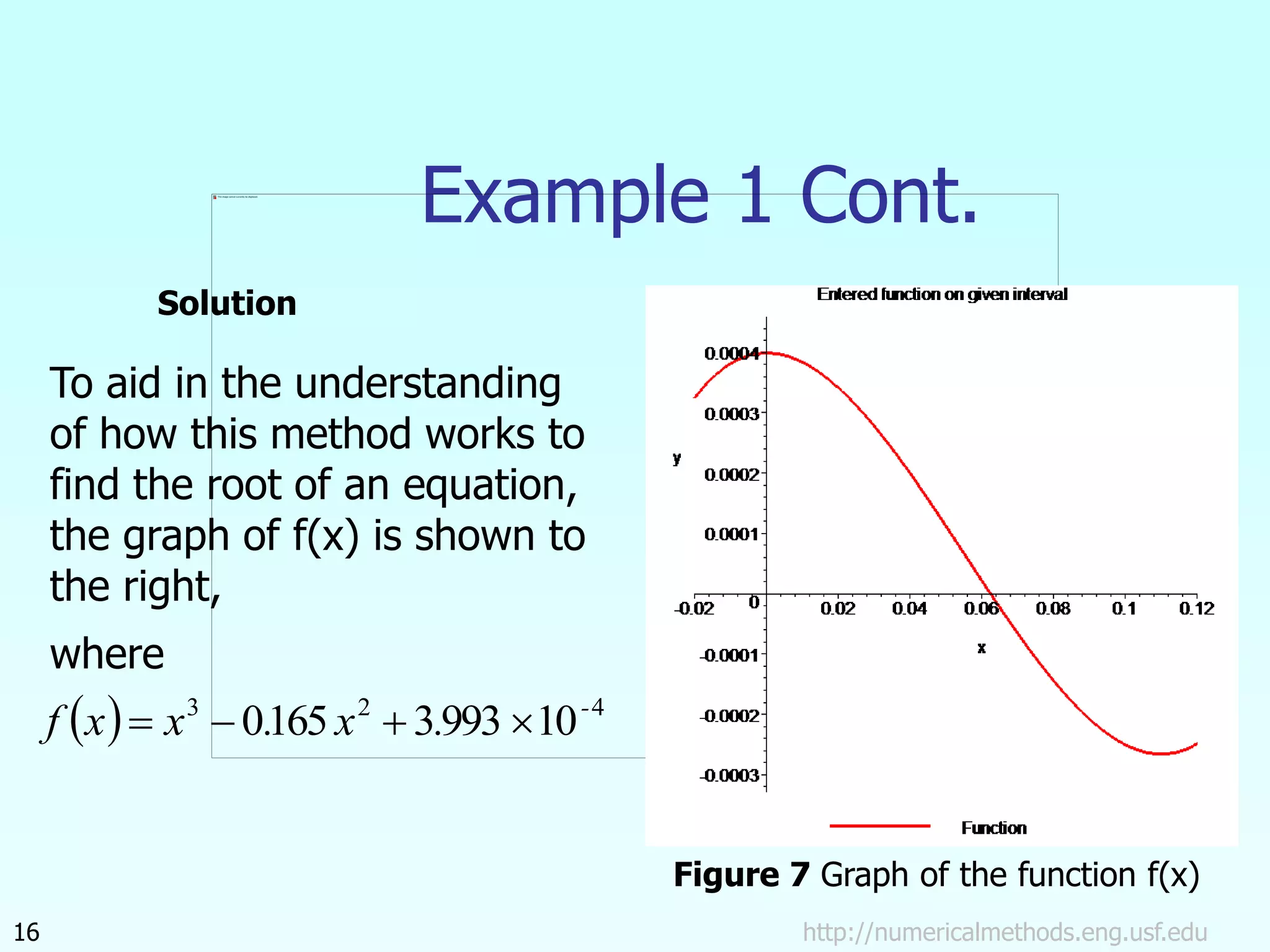
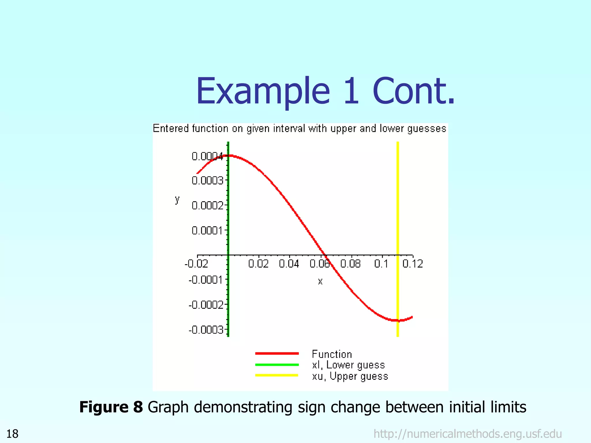
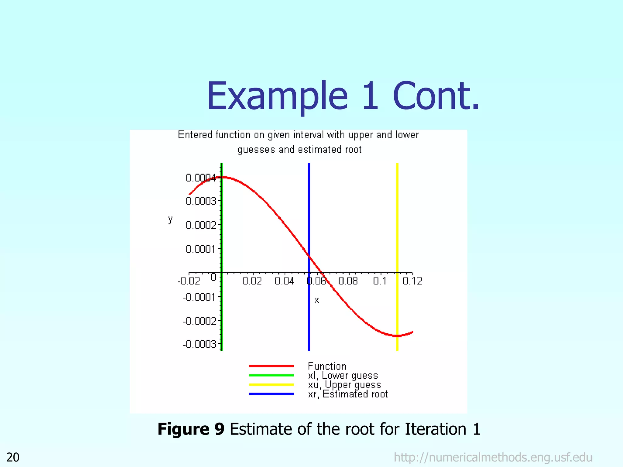
1. 8/11/2022 http://numericalmethods.eng.usf.edu 1
Bisection Method
Major: All Engineering Majors
Authors: Autar Kaw, Jai Paul
http://numericalmethods.eng.usf.edu
Transforming Numerical Methods Education for STEM
Undergraduates

2. Bisection Method
http://numericalmethods.eng.usf.edu

3. http://numericalmethods.eng.usf.edu
3
Basis of Bisection Method
Theorem
x
f(x)
xu
x
An equation f(x)=0, where f(x) is a real continuous function,
has at least one root between xl and xu if f(xl) f(xu) < 0.
Figure 1 At least one root exists between the two points if the function is
real, continuous, and changes sign.

4. x
f(x)
xu
x
http://numericalmethods.eng.usf.edu
4
Basis of Bisection Method
Figure 2 If function does not change sign between two
points, roots of the equation may still exist between the two
points.
 
x
f
  0

x
f

5. x
f(x)
xu
x
http://numericalmethods.eng.usf.edu
5
Basis of Bisection Method
Figure 3 If the function does not change sign between two
points, there may not be any roots for the equation between
the two points.
x
f(x)
xu
x
 
x
f
  0

x
f

6. x
f(x)
xu
x
http://numericalmethods.eng.usf.edu
6
Basis of Bisection Method
Figure 4 If the function changes sign between two points,
more than one root for the equation may exist between the two
points.
 
x
f
  0

x
f

7. http://numericalmethods.eng.usf.edu
7
Algorithm for Bisection Method

8. http://numericalmethods.eng.usf.edu
8
Step 1
Choose x and xu as two guesses for the root such that
f(x) f(xu) < 0, or in other words, f(x) changes sign
between x and xu. This was demonstrated in Figure 1.
x
f(x)
xu
x
Figure 1

9. x
f(x)
xu
x
xm
http://numericalmethods.eng.usf.edu
9
Step 2
Estimate the root, xm of the equation f (x) = 0 as the mid
point between x and xu as
x
x
m =
xu
 
2
Figure 5 Estimate of xm

10. http://numericalmethods.eng.usf.edu
10
Step 3
Now check the following
a) If , then the root lies between x and
xm; then x = x ; xu = xm.
b) If , then the root lies between xm and
xu; then x = xm; xu = xu.
c) If ; then the root is xm. Stop the
algorithm if this is true.
    0

m
l x
f
x
f
    0

m
l x
f
x
f
    0

m
l x
f
x
f

11. http://numericalmethods.eng.usf.edu
11
Step 4
x
x
m =
xu
 
2
100



 new
m
old
m
new
a
x
x
xm
root
of
estimate
current

new
m
x
root
of
estimate
previous

old
m
x
Find the new estimate of the root
Find the absolute relative approximate error
where

12. http://numericalmethods.eng.usf.edu
12
Step 5
Is ?
Yes
No
Go to Step 2 using new
upper and lower
guesses.
Stop the algorithm
Compare the absolute relative approximate error with
the pre-specified error tolerance .
a

s

s
a 

Note one should also check whether the number of
iterations is more than the maximum number of iterations
allowed. If so, one needs to terminate the algorithm and
notify the user about it.

13. http://numericalmethods.eng.usf.edu
13
Example 1
You are working for ‘DOWN THE TOILET COMPANY’ that
makes floats for ABC commodes. The floating ball has a
specific gravity of 0.6 and has a radius of 5.5 cm. You
are asked to find the depth to which the ball is
submerged when floating in water.
Figure 6 Diagram of the floating ball

14. http://numericalmethods.eng.usf.edu
14
Example 1 Cont.
The equation that gives the depth x to which the ball is
submerged under water is given by
a) Use the bisection method of finding roots of equations to
find the depth x to which the ball is submerged under
water. Conduct three iterations to estimate the root of
the above equation.
b) Find the absolute relative approximate error at the end
of each iteration, and the number of significant digits at
least correct at the end of each iteration.
0
10
993
.
3
165
.
0 4
2
3



 
x
x

15. http://numericalmethods.eng.usf.edu
15
Example 1 Cont.
From the physics of the problem, the ball would be
submerged between x = 0 and x = 2R,
where R = radius of the ball,
that is
 
11
.
0
0
055
.
0
2
0
2
0






x
x
R
x
Figure 6 Diagram of the floating ball

16. To aid in the understanding
of how this method works to
find the root of an equation,
the graph of f(x) is shown to
the right,
where
http://numericalmethods.eng.usf.edu
16
Example 1 Cont.
  4
2
3
10
993
3
165
0 -
.
x
.
x
x
f 



Figure 7 Graph of the function f(x)
Solution

17. http://numericalmethods.eng.usf.edu
17
Example 1 Cont.
Let us assume
11
.
0
00
.
0


u
x
x
Check if the function changes sign between x and xu .
       
        4
4
2
3
4
4
2
3
10
662
.
2
10
993
.
3
11
.
0
165
.
0
11
.
0
11
.
0
10
993
.
3
10
993
.
3
0
165
.
0
0
0



















f
x
f
f
x
f
u
l
Hence
           0
10
662
.
2
10
993
.
3
11
.
0
0 4
4





 

f
f
x
f
x
f u
l
So there is at least on root between x and xu, that is between 0 and 0.11

18. http://numericalmethods.eng.usf.edu
18
Example 1 Cont.
Figure 8 Graph demonstrating sign change between initial limits

19. http://numericalmethods.eng.usf.edu
19
Example 1 Cont.
055
.
0
2
11
.
0
0
2




 u
m
x
x
x 
       
           0
10
655
.
6
10
993
.
3
055
.
0
0
10
655
.
6
10
993
.
3
055
.
0
165
.
0
055
.
0
055
.
0
5
4
5
4
2
3
















f
f
x
f
x
f
f
x
f
m
l
m
Iteration 1
The estimate of the root is
Hence the root is bracketed between xm and xu, that is, between 0.055
and 0.11. So, the lower and upper limits of the new bracket are
At this point, the absolute relative approximate error cannot be
calculated as we do not have a previous approximation.
11
.
0
,
055
.
0 
 u
l x
x
a


20. http://numericalmethods.eng.usf.edu
20
Example 1 Cont.
Figure 9 Estimate of the root for Iteration 1

21. http://numericalmethods.eng.usf.edu
21
Example 1 Cont.
0825
.
0
2
11
.
0
055
.
0
2




 u
m
x
x
x 
       
         0
10
655
.
6
10
622
.
1
)
0825
.
0
(
055
.
0
10
622
.
1
10
993
.
3
0825
.
0
165
.
0
0825
.
0
0825
.
0
5
4
4
4
2
3


















f
f
x
f
x
f
f
x
f
m
l
m
Iteration 2
The estimate of the root is
Hence the root is bracketed between x and xm, that is, between 0.055
and 0.0825. So, the lower and upper limits of the new bracket are
0825
.
0
,
055
.
0 
 u
l x
x

22. http://numericalmethods.eng.usf.edu
22
Example 1 Cont.
Figure 10 Estimate of the root for Iteration 2

23. http://numericalmethods.eng.usf.edu
23
Example 1 Cont.
The absolute relative approximate error at the end of Iteration 2 is
a

%
333
.
33
100
0825
.
0
055
.
0
0825
.
0
100







 new
m
old
m
new
m
a
x
x
x
None of the significant digits are at least correct in the estimate root of
xm = 0.0825 because the absolute relative approximate error is greater
than 5%.

24. http://numericalmethods.eng.usf.edu
24
Example 1 Cont.
06875
.
0
2
0825
.
0
055
.
0
2




 u
m
x
x
x 
       
           0
10
563
.
5
10
655
.
6
06875
.
0
055
.
0
10
563
.
5
10
993
.
3
06875
.
0
165
.
0
06875
.
0
06875
.
0
5
5
5
4
2
3


















f
f
x
f
x
f
f
x
f
m
l
m
Iteration 3
The estimate of the root is
Hence the root is bracketed between x and xm, that is, between 0.055
and 0.06875. So, the lower and upper limits of the new bracket are
06875
.
0
,
055
.
0 
 u
l x
x

25. http://numericalmethods.eng.usf.edu
25
Example 1 Cont.
Figure 11 Estimate of the root for Iteration 3

26. http://numericalmethods.eng.usf.edu
26
Example 1 Cont.
The absolute relative approximate error at the end of Iteration 3 is
a

%
20
100
06875
.
0
0825
.
0
06875
.
0
100







 new
m
old
m
new
m
a
x
x
x
Still none of the significant digits are at least correct in the estimated
root of the equation as the absolute relative approximate error is
greater than 5%.
Seven more iterations were conducted and these iterations are shown in
Table 1.

27. http://numericalmethods.eng.usf.edu
27
Table 1 Cont.
Table 1 Root of f(x)=0 as function of number of iterations for
bisection method.
Iteration x xu xm a % f(xm)
1
2
3
4
5
6
7
8
9
10
0.00000
0.055
0.055
0.055
0.06188
0.06188
0.06188
0.06188
0.0623
0.0623
0.11
0.11
0.0825
0.06875
0.06875
0.06531
0.06359
0.06273
0.06273
0.06252
0.055
0.0825
0.06875
0.06188
0.06531
0.06359
0.06273
0.0623
0.06252
0.06241
----------
33.33
20.00
11.11
5.263
2.702
1.370
0.6897
0.3436
0.1721
6.655×10−5
−1.622×10−4
−5.563×10−5
4.484×10−6
−2.593×10−5
−1.0804×10−5
−3.176×10−6
6.497×10−7
−1.265×10−6
−3.0768×10−7

28. http://numericalmethods.eng.usf.edu
28
Table 1 Cont.
Hence the number of significant digits at least correct is given by the
largest value or m for which
 
  463
.
2
3442
.
0
log
2
2
3442
.
0
log
10
3442
.
0
10
5
.
0
1721
.
0
10
5
.
0
2
2
2














m
m
m
m
m
a
2

m
So
The number of significant digits at least correct in the estimated root
of 0.06241 at the end of the 10th iteration is 2.

29. http://numericalmethods.eng.usf.edu
29
Advantages
 Always convergent
 The root bracket gets halved with each
iteration - guaranteed.

30. http://numericalmethods.eng.usf.edu
30
Drawbacks
 Slow convergence
 If one of the initial guesses is close to
the root, the convergence is slower

31. http://numericalmethods.eng.usf.edu
31
Drawbacks (continued)
 If a function f(x) is such that it just
touches the x-axis it will be unable to find
the lower and upper guesses.
f(x)
x
  2
x
x
f 

32. http://numericalmethods.eng.usf.edu
32
Drawbacks (continued)
 Function changes sign but root does not
exist
f(x)
x
 
x
x
f
1


33. Additional Resources
For all resources on this topic such as digital audiovisual
lectures, primers, textbook chapters, multiple-choice
tests, worksheets in MATLAB, MATHEMATICA, MathCad
and MAPLE, blogs, related physical problems, please
visit
http://numericalmethods.eng.usf.edu/topics/bisection_
method.html

34. THE END
http://numericalmethods.eng.usf.edu