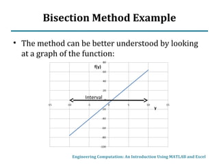
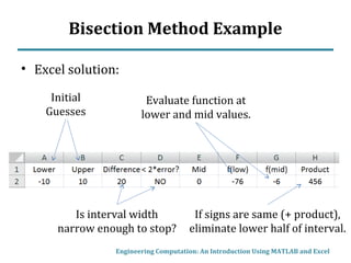
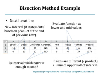
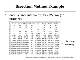
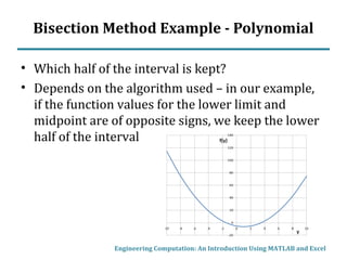
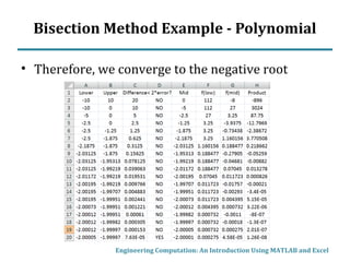
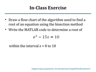
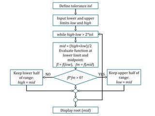
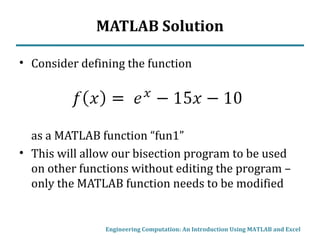
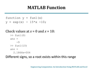
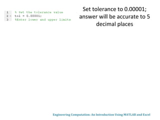
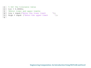
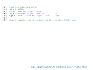
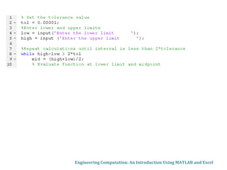
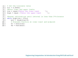
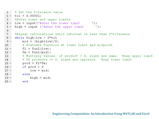
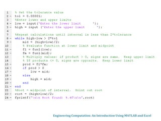
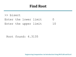
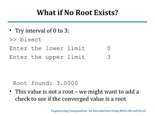
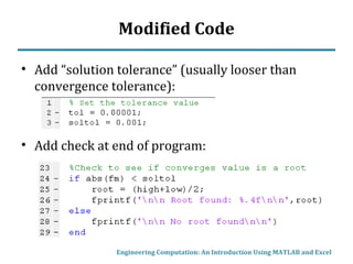
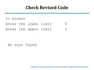
This document describes the bisection method for finding roots of equations numerically. It begins by classifying equations as linear, polynomial, or generally non-linear. For non-linear equations, numerical methods are required. The bisection method iteratively halves the interval that contains a root until a solution is found to within a specified tolerance. An example illustrates the step-by-step process of applying the bisection method to find the root of a sample function. MATLAB code is also presented to implement the bisection method.

1. Chapter 6
Finding the Roots of
Equations
The Bisection Method
Copyright © The McGraw-Hill Companies, Inc. Permission required for reproduction or display.

2. Finding Roots of Equations
• In this chapter, we are examining equations with
one independent variable.
• These equations may be linear or non-linear
• Non-linear equations may be polynomials or
generally non-linear equations
• A root of the equation is simply a value of the
independent variable that satisfies the equation
Engineering Computation: An Introduction Using MATLAB and Excel

3. Classification of Equations
• Linear: independent variable appears to the first
power only, either alone or multiplied by a
constant
• Nonlinear:
– Polynomial: independent variable appears
raised to powers of positive integers only
– General non-linear: all other equations
Engineering Computation: An Introduction Using MATLAB and Excel

4. Finding Roots of Equations
• As with our method for solving simultaneous non-
linear equations, we often set the equation to be
equal to zero when the equation is satisfied
• Example:
• If we say that
then when f(y) =0, the equation is satisfied
Engineering Computation: An Introduction Using MATLAB and Excel

5. Solution Methods
• Linear: Easily solved analytically
• Polynomials: Some can be solved analytically
(such as by quadratic formula), but most will
require numerical solution
• General non-linear: unless very simple, will
require numerical solution
Engineering Computation: An Introduction Using MATLAB and Excel

6. The Bisection Method
• In the bisection method, we start with an interval
(initial low and high guesses) and halve its width
until the interval is sufficiently small
• As long as the initial guesses are such that the
function has opposite signs at the two ends of the
interval, this method will converge to a solution
• Example: Consider the function
Engineering Computation: An Introduction Using MATLAB and Excel

7. Bisection Method Example
• Consider an initial interval of ylower = -10 to yupper = 10
• Since the signs are opposite, we know that the
method will converge to a root of the equation
• The value of the function at the midpoint of the
interval is:
Engineering Computation: An Introduction Using MATLAB and Excel

8. Bisection Method Example
• The method can be better understood by looking
at a graph of the function:
Engineering Computation: An Introduction Using MATLAB and Excel
Interval

9. Bisection Method Example
• Now we eliminate half of the interval, keeping the
half where the sign of f(midpoint) is opposite the
sign of f(endpoint)
• In this case, since f(ymid) = -6 and f(yupper) = 64, we
keep the upper half of the interval, since the
function crosses zero in this interval
Engineering Computation: An Introduction Using MATLAB and Excel

10. Bisection Method Example
• Now we eliminate half of the interval, keeping the
half where the sign of f(midpoint) is opposite the
sign of f(endpoint)
• In this case, since f(ymid) = -6 and f(yupper) = 64, we
keep the upper half of the interval, since the
function crosses zero in this interval
Engineering Computation: An Introduction Using MATLAB and Excel

11. Bisection Method Example
• The interval has now been bisected, or halved:
Engineering Computation: An Introduction Using MATLAB and Excel
New Interval

12. Bisection Method Example
• New interval: ylower = 0, yupper = 10, ymid = 5
• Function values:
• Since f(ylower) and f(ymid) have opposite signs, the
lower half of the interval is kept
Engineering Computation: An Introduction Using MATLAB and Excel

13. Bisection Method Example
• At each step, the difference between the high and
low values of y is compared to 2*(allowable error)
• If the difference is greater, than the procedure
continues
• Suppose we set the allowable error at 0.0005. As
long as the width of the interval is greater than
0.001, we will continue to halve the interval
• When the width is less than 0.001, then the
midpoint of the range becomes our answer
Engineering Computation: An Introduction Using MATLAB and Excel

14. Bisection Method Example
• Excel solution:
Engineering Computation: An Introduction Using MATLAB and Excel
Initial
Guesses
Is interval width
narrow enough to stop?
Evaluate function at
lower and mid values.
If signs are same (+ product),
eliminate lower half of interval.

15. Bisection Method Example
• Next iteration:
Engineering Computation: An Introduction Using MATLAB and Excel
New Interval (if statements
based on product at the end
of previous row)
Is interval width narrow
enough to stop?
Evaluate function at
lower and mid values.
If signs are different (- product),
eliminate upper half of interval.

16. Bisection Method Example
• Continue until interval width < 2*error (16
iterations)
Engineering Computation: An Introduction Using MATLAB and Excel
Answer:
y = 0.857

17. Bisection Method Example
• Or course, we know that the exact answer is 6/7
(0.857143)
• If we wanted our answer accurate to 5 decimal
places, we could set the allowable error to
0.000005
• This increases the number of iterations only from
16 to 22 – the halving process quickly reduces the
interval to very small values
• Even if the initial guesses are set to -10,000 and
10000, only 32 iterations are required to get a
solution accurate to 5 decimal places
Engineering Computation: An Introduction Using MATLAB and Excel

18. Bisection Method Example - Polynomial
• Now consider this example:
• Use the bisection method, with allowed error of
0.0001
Engineering Computation: An Introduction Using MATLAB and Excel

19. Bisection Method Example - Polynomial
• If limits of -10 to 0
are selected, the
solution converges
to x = -2
Engineering Computation: An Introduction Using MATLAB and Excel

20. Bisection Method Example - Polynomial
• If limits of 0 to 10
are selected, the
solution converges
to x = 4
Engineering Computation: An Introduction Using MATLAB and Excel

21. Bisection Method Example - Polynomial
• If limits of -10 to 10 are selected, which root is
found?
• In this case f(-10) and f(10) are both positive, and
f(0) is negative
Engineering Computation: An Introduction Using MATLAB and Excel

22. Bisection Method Example - Polynomial
• Which half of the interval is kept?
• Depends on the algorithm used – in our example,
if the function values for the lower limit and
midpoint are of opposite signs, we keep the lower
half of the interval
Engineering Computation: An Introduction Using MATLAB and Excel

23. Bisection Method Example - Polynomial
• Therefore, we converge to the negative root
Engineering Computation: An Introduction Using MATLAB and Excel

24. In-Class Exercise
• Draw a flow chart of the algorithm used to find a
root of an equation using the bisection method
• Write the MATLAB code to determine a root of
within the interval x = 0 to 10
Engineering Computation: An Introduction Using MATLAB and Excel

25. Input lower and upper
limits low and high
Define tolerance tol
while high-low > 2*tol
mid = (high+low)/2
Evaluate function at
lower limit and
midpoint:
fl = f(low), fm = f(mid)
fl*fm > 0?
Keep upper half of
range:
low = mid
Keep lower half
of range:
high = mid
Display root (mid)
YESNO

26. MATLAB Solution
• Consider defining the function
as a MATLAB function “fun1”
• This will allow our bisection program to be used
on other functions without editing the program –
only the MATLAB function needs to be modified
Engineering Computation: An Introduction Using MATLAB and Excel

27. MATLAB Function
function y = fun1(x)
y = exp(x) - 15*x -10;
Check values at x = 0 and x = 10:
>> fun1(0)
ans =
-9
>> fun1(10)
ans =
2.1866e+004
Different signs, so a root exists within this range
Engineering Computation: An Introduction Using MATLAB and Excel

28. Engineering Computation: An Introduction Using MATLAB and Excel
Set tolerance to 0.00001;
answer will be accurate to 5
decimal places

29. Engineering Computation: An Introduction Using MATLAB and Excel

30. Engineering Computation: An Introduction Using MATLAB and Excel

31. Engineering Computation: An Introduction Using MATLAB and Excel

32. Engineering Computation: An Introduction Using MATLAB and Excel

33. Engineering Computation: An Introduction Using MATLAB and Excel

34. Engineering Computation: An Introduction Using MATLAB and Excel

35. Find Root
>> bisect
Enter the lower limit 0
Enter the upper limit 10
Root found: 4.3135
Engineering Computation: An Introduction Using MATLAB and Excel

36. What if No Root Exists?
• Try interval of 0 to 3:
>> bisect
Enter the lower limit 0
Enter the upper limit 3
Root found: 3.0000
• This value is not a root – we might want to add a
check to see if the converged value is a root
Engineering Computation: An Introduction Using MATLAB and Excel

37. Modified Code
• Add “solution tolerance” (usually looser than
convergence tolerance):
• Add check at end of program:
Engineering Computation: An Introduction Using MATLAB and Excel

38. Check Revised Code
>> bisect
Enter the lower limit 0
Enter the upper limit 3
No root found
Engineering Computation: An Introduction Using MATLAB and Excel

39. Numerical Tools
• Of course, Excel and MATLAB have built-in tools
for finding roots of equations
• However, the examples we have considered
illustrate an important concept about non-linear
solutions:
Remember that there may be many roots to a
non-linear equation. Even when specifying an
interval to be searched, keep in mind that there
may be multiple solutions (or no solution) within
the interval.
Engineering Computation: An Introduction Using MATLAB and Excel