Downloaded 387 times


![Questions
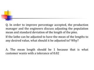
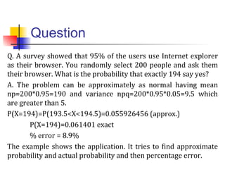
Q. What percentage of pins will be accepted by the
customer?
A. Required Percentage =
(NORM.DIST(1.02,1.012,0.018,TRUE)-
NORM.DIST(0.98,1.012,0.018,TRUE))
= 0.633919177 [ Using MS Excel ]
It means that around 63.4% of the nails will be accepted
by the customer.](https://image.slidesharecdn.com/687ee170-5515-4689-accf-2f67d0cbf082-150527083207-lva1-app6892/85/Normal-Distribution-61-320.jpg)


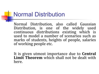
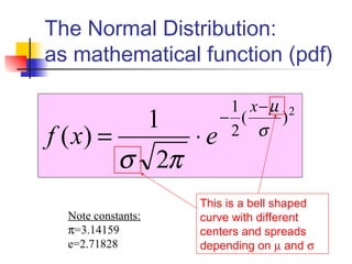
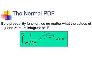
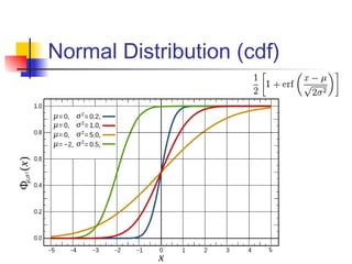
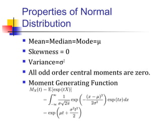
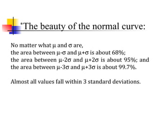
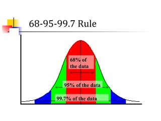
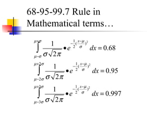
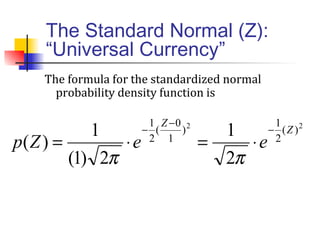
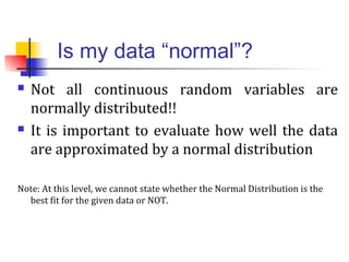
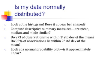
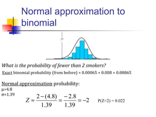
This document discusses the normal distribution and related concepts. It begins with an introduction to the normal distribution and its properties. It then covers the probability density function and cumulative distribution function of the normal distribution. The rest of the document discusses key properties like the 68-95-99.7 rule, using the standard normal distribution, and how to determine if a data set follows a normal distribution including using a normal probability plot. Examples are provided throughout to illustrate the concepts.
![AP Stats Chapter 1 Exploring Data [Autosaved] (1).ppt](https://cdn.slidesharecdn.com/ss_thumbnails/apstatschapter1exploringdataautosaved1-240908213027-9f0b3ffa-thumbnail.jpg?width=640&height=640&fit=bounds)