2
When computing probabilitiesfor discrete
random variables, we usually substitute the
value of the random variable into a formula.
However, this is not the same for continuous
variables since they can take up infinite
values within an interval.
3.
PROBABILITY DENSITY FUNCTION
Probability3
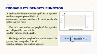
A probability density function (pdf) is an equation
used to compute probabilities of
continuous random variables. It must satisfy the
following two rules:
1. The total area under the graph of the equation
over all possible values of the
random variable must equal 1.
2. The height of the graph of the equation must be
greater than or equal to 0 for all
possible values of the random variable.
𝑃 = න
−∞
∞
𝑓(𝑥) 𝑑𝑥 = 1
4.
PROBABILITY DENSITY FUNCTION
Probability4
Unlike the case of discrete random variables, for a continuous random variable any
single outcome has probability zero of occurring. (ex. P(x=1)=0)
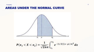
The probability that a random variable X takes a value in the interval [a,b] is
given by the function f(x)
𝑃 𝑎 ≤ 𝑋 ≤ 𝑏 = න
𝑎
𝑏
𝑓(𝑥) 𝑑𝑥
The area under the graph of a density
function over an interval represents the
probability of observing a value of the
random variable in that interval.
UNIFORM PROBABILITY DISTRIBUTION
Probability6
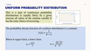
This is a type of continuous probability
distributions is equally likely. In a given
interval, all values of the random variable X
has the same chance of occurring.
The probability density function of a uniform distribution is a constant.
𝑓 𝑥 =
1
𝑏 − 𝑎
Where b=upper limit, a=lower limit.
𝜇 =
𝑎+𝑏
2
𝜎 =
𝑏−𝑎 2
12
7.
EXAMPLE
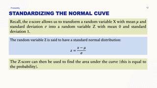
Suppose that alarge conference room for a
certain company can be reserved for no more
than 4 hours. However, the use of the conference
room is such that both long and short
conferences occur quite often. In fact, it can be
assumed that length X of a conference has a
uniform distribution on the interval [0, 4].
What is the probability density function?
What is the probability that any given conference
lasts at least 3 hours?
Presentation title 7
NORMAL PROBABILITY DISTRIBUTION
Probability9
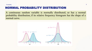
A continuous random variable is normally distributed, or has a normal
probability distribution, if its relative frequency histogram has the shape of a
normal curve.
10.
PROPERTIES OF THENORMAL CURVE
Probability 10
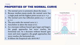
1. The normal curve is symmetric about the mean.
2. Because median=mean=mode, the normal curve has
a single peak and the highest point occurs at 𝑥 = 𝜇
3. The normal curve has inflection points at 𝜇 − 𝜎 and
𝜇 + 𝜎
4. The area under the normal curve is 1.
5. Area below or above the mean is 0.5.
6. As x increases without bound (gets larger and larger),
the graph approaches but never reaches, the
horizontal axis. As x decreases without bound (gets
more and more negative), the graph approaches, but
never reaches, the horizontal axis.
7. It follows the Empirical rule: 68-95-99.7
STANDARDIZING THE NORMALCUVE
Probability 12
The random variable Z is said to have a standard normal distribution:
𝑧 =
𝑥 − 𝜇
𝜎
Recall, the z-score allows us to transform a random variable X with mean µ and
standard deviation σ into a random variable Z with mean 0 and standard
deviation 1.
The Z-score can then be used to find the area under the curve (this is equal to
the probability).
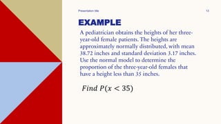
13.
EXAMPLE
A pediatrician obtainsthe heights of her three-
year-old female patients. The heights are
approximately normally distributed, with mean
38.72 inches and standard deviation 3.17 inches.
Use the normal model to determine the
proportion of the three-year-old females that
have a height less than 35 inches.
Presentation title 13
𝐹𝑖𝑛𝑑 𝑃(𝑥 < 35)
14.
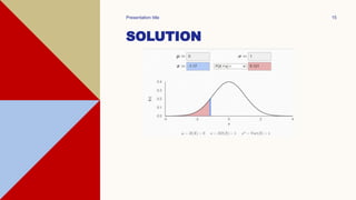
SOLUTION
Find the correspondingZ-score
𝑧 =
35 − 38.72
3.17
= −1.17
Since we are interested with P(x<35), we want
the area to the left of the z-score.
Presentation title 14
EXAMPLE
A pediatrician obtainsthe heights of her three-
year-old female patients. The heights are
approximately normally distributed, with mean
38.72 inches and standard deviation 3.17 inches.
Use the normal model to determine the
proportion of the three-year-old females that
have a height greater than 39 inches.
Presentation title 16
𝐹𝑖𝑛𝑑 𝑃(𝑥 > 39)
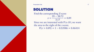
17.
SOLUTION
Find the correspondingZ-score
𝑧 =
39 − 38.72
3.17
= 0.09
Since we are interested with P(x>39), we want
the area to the right of the z-score.
P 𝑧 > 0.09 = 1 − 0.53586 = 0.46414
Presentation title 17
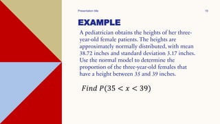
EXAMPLE
A pediatrician obtainsthe heights of her three-
year-old female patients. The heights are
approximately normally distributed, with mean
38.72 inches and standard deviation 3.17 inches.
Use the normal model to determine the
proportion of the three-year-old females that
have a height between 35 and 39 inches.
Presentation title 19
𝐹𝑖𝑛𝑑 𝑃(35 < 𝑥 < 39)
20.
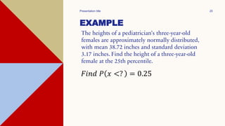
EXAMPLE
The heights ofa pediatrician’s three-year-old
females are approximately normally distributed,
with mean 38.72 inches and standard deviation
3.17 inches. Find the height of a three-year-old
female at the 25th percentile.
Presentation title 20
𝐹𝑖𝑛𝑑 𝑃 𝑥 <? = 0.25
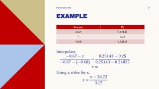
21.
EXAMPLE
Z-score Pz
-0.67 0.25143
?0.25
-0.68 0.24825
Presentation title 21
Interpolate
−0.67 − 𝑧
−0.67 − (−0.68)
=
0.25143 − 0.25
0.25143 − 0.24825
𝑧 =
Using z, solve for x.
𝑧 =
𝑥 − 38.72
3.17
22.
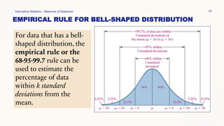
EMPIRICAL RULE FORBELL-SHAPED DISTRIBUTION
Descriptive Statistics – Measures of Dispersion 22
For data that has a bell-
shaped distribution, the
empirical rule or the
68-95-99.7 rule can be
used to estimate the
percentage of data
within k standard
deviations from the
mean.
23.
EXAMPLE
Descriptive Statistics 23
Givena bell-shaped distribution with a sample mean of
40 and a standard deviation of 10,
a) What is the percentage of observations that will have
a value between 20 and 60?
b) What is the percentage of observations that has a
value less than 10 and greater than 60?
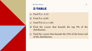
24.
Z-TABLE
Descriptive Statistics 24
a)Find P(z> 2.12)
b) Find P(z<-0.89)
c) Find P(0.12<z<1.88)
d) Find the z-score that bounds the top 9% of the
distribution.
e) Find the z-score that bounds the 25% of the lower tail
of the distribution.
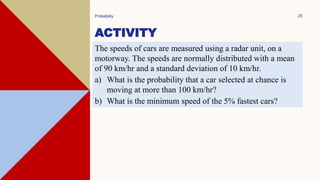
25.
ACTIVITY
Probability 25
The speedsof cars are measured using a radar unit, on a
motorway. The speeds are normally distributed with a mean
of 90 km/hr and a standard deviation of 10 km/hr.
a) What is the probability that a car selected at chance is
moving at more than 100 km/hr?
b) What is the minimum speed of the 5% fastest cars?
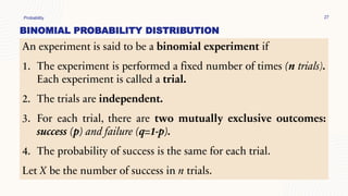
BINOMIAL PROBABILITY DISTRIBUTION
Probability27
An experiment is said to be a binomial experiment if
1. The experiment is performed a fixed number of times (n trials).
Each experiment is called a trial.
2. The trials are independent.
3. For each trial, there are two mutually exclusive outcomes:
success (p) and failure (q=1-p).
4. The probability of success is the same for each trial.
Let X be the number of success in n trials.
28.
28
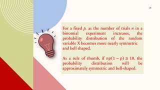
For a fixedp, as the number of trials n in a
binomial experiment increases, the
probability distribution of the random
variable X becomes more nearly symmetric
and bell shaped.
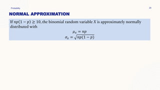
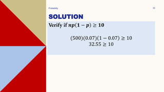
As a rule of thumb, if 𝑛𝑝 1 − 𝑝 ≥ 10, the
probability distribution will be
approximately symmetric and bell-shaped.
Normal Probability 30
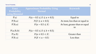
Exact
Probability
usingBinomial
Approximate Probability Using
Normal
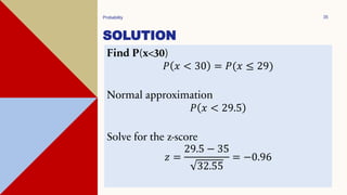
Keywords
P(a) 𝑃(𝑎 − 0.5 ≤ 𝑋 ≤ 𝑎 + 0.5) Equal to
P(X≤a) 𝑃(𝑋 ≤ 𝑎 + 0.5) At most, less than or equal to
P(X≥a) 𝑃(𝑎 − 0.5 ≤ 𝑋) At least, greater than or equal
to
P(a≤X≤b) 𝑃(𝑎 − 0.5 ≤ 𝑋 ≤ 𝑏 + 0.5)
P(a<X) 𝑃(𝑎 + 0.5 < 𝑋) Greater than
P(X<a) 𝑃(𝑋 < 𝑎 − 0.5) Less than
31.
EXAMPLE
Probability 31
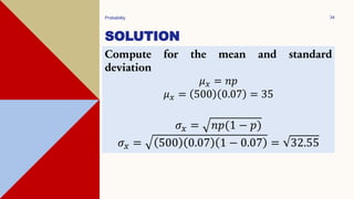
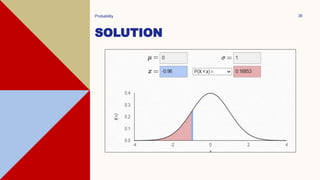
According tothe American Red Cross, 7% of
people in the United States have blood type O-
negative. What is the probability that, in a
simple random sample of 500 people in the
United States, fewer than 30 have blood type
O-negative?
EXAMPLE
Probability 37
What isthe probability that, in a simple random
sample of 500 people in the United States, 20
have blood type O-negative?
38.
ACTIVITY
Probability 38
A home-basedbaker was able to produce 200 cupcakes
within 8 hours of operation. In average, the cupcakes weigh
110 grams with a standard deviation 10 grams. To be
considered acceptable to the buyer, a cupcake should weigh
within 2 standard deviations from the mean. Historically, 5%
of the cupcakes do not pass the standard weight. To test for
consistency, you randomly sampled 15 cupcakes, what is the
probability that at most 7 will pass the standard weight?
POISSON DISTRIBUTION
Probability 40
ThePoisson probability distribution can be used to
compute probabilities of experiments in which the
random variable X counts the number of
occurrences (successes) of a particular event
within a specified interval (usually time or space).
Where λ (the Greek letter lambda) represents the
average number of occurrences of the event in some
interval length.
41.
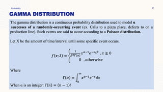
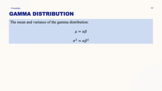
GAMMA DISTRIBUTION
Probability 41
Thegamma distribution is a continuous probability distribution used to model α
successes of a randomly-occurring event (ex. Calls to a pizza place, defects to on a
production line). Such events are said to occur according to a Poisson distribution.
Let X be the amount of time/interval until some specific event occurs.
𝑓 𝑥; 𝜆 = ቐ
1
𝛽𝛼Γ(𝛼)
𝑥𝛼−1𝑒−𝑥/𝛽 , 𝑥 ≥ 0
0 , 𝑜𝑡ℎ𝑒𝑟𝑤𝑖𝑠𝑒
Where
Γ 𝛼 = න
0
∞
𝑥𝛼−1𝑒−𝑥𝑑𝑥
When α is an integer: Γ 𝑛 = 𝑛 − 1 !
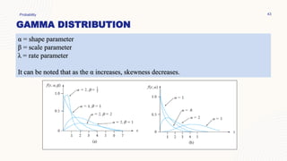
GAMMA DISTRIBUTION
Probability 43
α= shape parameter
β = scale parameter
λ = rate parameter
It can be noted that as the α increases, skewness decreases.
44.
EXAMPLE
Probability 44
On aSaturday morning, customers arrive at a
bakery according to a Poisson process at an
average rate of 15 per hour.
What is the probability that it takes less than 10
minutes for the first 3 customers?
45.
EXAMPLE
Probability 45
On aSaturday morning, customers arrive at a
bakery according to a Poisson process at an
average rate of 15 per hour.
What is the average amount of time that will
elapse before 3 customers arrive in the bakery?
46.
EXAMPLE
Probability 46
On aSaturday morning, customers arrive at a
bakery according to a Poisson process at an
average rate of 15 per hour.
What is the probability that exactly 15 customers
arrive in an hour?
47.
EXAMPLE
Probability 47
In acertain city, the daily consumption of
electric power, in millions of kilowatt-hours,
is a random variable X having a gamma
distribution with mean µ = 6 and variance σ2
= 12.
a. Find the values of α and β.
b. Find the probability that on any given day
the daily power consumption will exceed
12 million kilowatthours.
48.
ACTIVITY
Probability 48
Suppose thatwhen a transistor of a certain
type is subjected to an accelerated life test, the
lifetime X (in weeks) has a gamma
distribution with mean of 24 weeks and
standard deviation of 12 weeks.
a) What is the probability that a transistor
will last between 12 and 24 weeks?
b) What is the probability that a transistor
will last at most 24 weeks?
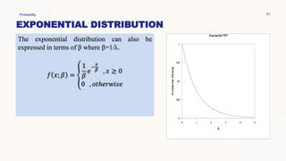
EXPONENTIAL DISTRIBUTION
Probability 50
Theexponential distribution is a special case of a gamma distribution where α=1
Let X be the amount of time/interval until some specific event occurs and λ is the average
number of occurrences in an interval.
𝑓 𝑥; 𝜆 = ቊ𝜆𝑒−𝜆𝑥 , 𝑥 ≥ 0
0 , 𝑜𝑡ℎ𝑒𝑟𝑤𝑖𝑠𝑒
• The exponential distribution generally have fewer large values and more small values.
• The exponential distribution has the following mean and variance:
𝜇 =
1
𝜆
𝜎2
=
1
𝜆2
EXAMPLE
Probability 52
Data collectedat Toronto Pearson International
Airport suggests that an exponential
distribution with mean value 2.725 hours is a
good model for rainfall duration.
What is the probability that the duration of a
particular rainfall event at this location is
• at least 2 hours?
• At most 3 hours?
• Between 2 and 3 hours?
53.
ACTIVITY
Probability 53
Let Xdenote the distance (m) that an animal
moves from its birth site to the first territorial
vacancy it encounters. Suppose that for banner-
tailed kangaroo rats, X has an exponential
distribution with parameter λ=0.01386.
a. What is the probability that the distance is at
most 100 m?
b. At most 200 m?
c. Between 100 and 200 m?


![PROBABILITY DENSITY FUNCTION
Probability 4
Unlike the case of discrete random variables, for a continuous random variable any
single outcome has probability zero of occurring. (ex. P(x=1)=0)
The probability that a random variable X takes a value in the interval [a,b] is
given by the function f(x)
𝑃 𝑎 ≤ 𝑋 ≤ 𝑏 = න
𝑎
𝑏
𝑓(𝑥) 𝑑𝑥
The area under the graph of a density
function over an interval represents the
probability of observing a value of the
random variable in that interval.](https://image.slidesharecdn.com/module6-continuousdistributionefcd52595b081d24a9bc3ca31b5f8d05-250303223331-da7f94ce/85/Module-6-Continuous-Distribution_efcd52595b081d24a9bc3ca31b5f8d05-pdf-4-320.jpg)

![EXAMPLE
Suppose that a large conference room for a
certain company can be reserved for no more
than 4 hours. However, the use of the conference
room is such that both long and short
conferences occur quite often. In fact, it can be
assumed that length X of a conference has a
uniform distribution on the interval [0, 4].
What is the probability density function?
What is the probability that any given conference
lasts at least 3 hours?
Presentation title 7](https://image.slidesharecdn.com/module6-continuousdistributionefcd52595b081d24a9bc3ca31b5f8d05-250303223331-da7f94ce/85/Module-6-Continuous-Distribution_efcd52595b081d24a9bc3ca31b5f8d05-pdf-7-320.jpg)