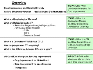
This document provides an overview of molecular markers and quantitative trait locus (QTL) mapping. It begins with a discussion of different types of genetic variation and how molecular markers can be used to detect variation at the DNA level. The document then describes different types of molecular markers, including restriction fragment length polymorphisms (RFLPs), polymerase chain reaction (PCR)-based markers, simple sequence repeats (SSRs), and single nucleotide polymorphisms (SNPs). It also discusses what a QTL is and how QTL mapping is performed. The document concludes with how molecular markers and QTL mapping can be used to understand the genetic basis of traits and help improve crops.

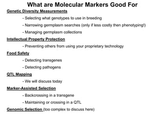
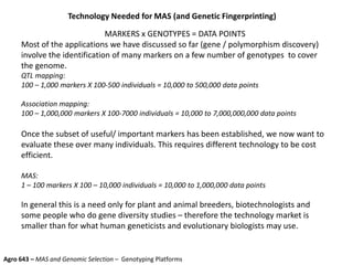
![What is a Marker?
-Websters Dictionary defines as:
“…something that serves to identify, predict, or characterize […the
GENETIC VARIATION present]”
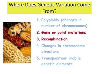
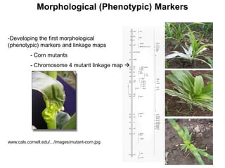
Morphological (phenotypic) markers
- A trait you can observe and/or measure as different between two
individuals (must be heritable, genetic). (Example ~ corn mutants)
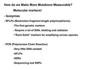
Genetic (molecular, DNA) markers
- A measurable DNA mutation which may or may not have an effect
on the phenotype (also must be heritable, genetic).
Molecular markers are much more common than phenotypic markers
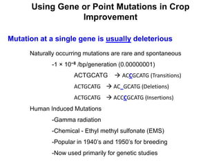
Most gene (point) mutations do not result in phenotypic changes.
www.cals.cornell.edu/.../images/mutant-corn.jpg](https://image.slidesharecdn.com/molecularquantitativegeneticsforplantbreedingroundtable2010x-160526071328/85/Molecular-quantitative-genetics-for-plant-breeding-roundtable-2010x-8-320.jpg)


![谷歌留痕技术 [ 𝙩𝙤𝙥 𝟮𝟯𝟯. 𝙘 𝙤𝙢 ]](https://cdn.slidesharecdn.com/ss_thumbnails/top233-260130174328-3833018c-thumbnail.jpg?width=640&height=640&fit=bounds)


