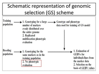
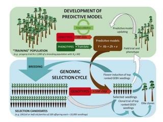
Introduction: Proposed by Meuwissen et al. (2001) GS is a specialized form of MAS, in which information from genotype data on marker alleles covering the entire genome forms the basis of selection. The effects associated with all the marker loci, irrespective of whether the effects are significant or not, covering the entire genome are estimated. The marker effect estimates are used to calculate the genomic estimated breeding values (GEBVs) of different individuals/lines, which form the basis of selection. Why to go for genomic selection: Marker-assisted selection (MAS) is well-suited for handling oligogenes and quantitative trait loci (QTLs) with large effects but not for minor QTLs. MARS attempts to take into account small effect QTLs by combining trait phenotype data with marker genotype data into a combined selection index. Based on markers showing significant association with the trait(s) and for this reason has been criticized as inefficient The genomic selection (GS) scheme was to rectify the deficiency of MAS and MARS schemes. The GS scheme utilizes information from genome-wide marker data whether or not their associations with the concerned trait(s) are significant. GEBV: GenomicEstimated Breeding Values- The sum total of effects associated with all the marker alleles present in the individual and included in the GS model applied to the population under selection Calculated on a single individual basis Gene-assisted genomic selection: A GS model that uses information about prior known QTLs, the targeted QTLs were accumulated in much higher frequencies than when the standard ridge regression was used The sum total of effects associated with all the marker alleles present in the individual and included in the GS model applied to the population under selection Calculated on a single individual basis Population used: Training population: used for training of the GS model and for obtaining estimates of the marker-associated effects needed for estimation of GEBVs of individuals/lines in the breeding population. Breeding population: the population subjected to GS for achieving the desired improvement and isolation of superior lines for use as new varieties/parents of new improved hybrids. Training population- large enough: must be representative of the breeding population: max. trait variance with marker : by cluster analysis should have either equal or comparable LD, LD decay rates with breeding populations Updated by including individuals/lines from the breeding population Training more than one generation Low colinearity between markers is needed since high colinearity tends to reduce prediction accuracy of certain GS models. (colinearity disturbed by recombination)

1. Genomic Selection
Presented by
Debadatta Panda

2. Introduction
• Proposed by Meuwissen et al. (2001)
• GS is a specialized form of MAS, in which information
from genotype data on marker alleles covering the
entire genome forms the basis of selection.
• The effects associated with all the marker loci,
irrespective of whether the effects are significant or
not, covering the entire genome are estimated.
• The marker effect estimates are used to calculate the
genomic estimated breeding values (GEBVs) of
different individuals/lines, which form the basis of
selection.

3. Why to go for genomic selection
• Marker-assisted selection (MAS) is well-suited for handling
oligogenes and quantitative trait loci (QTLs) with large effects
but not for minor QTLs.
• MARS attempts to take into account small effect QTLs by
combining trait phenotype data with marker genotype data
into a combined selection index.
• Based on markers showing significant association with the
trait(s) and for this reason has been criticized as inefficient
• The genomic selection (GS) scheme was to rectify the
deficiency of MAS and MARS schemes. The GS scheme utilizes
information from genome-wide marker data whether or not
their associations with the concerned trait(s) are significant.

4. GEBV: Genomic
Estimated Breeding Values
• The sum total of effects associated with all the
marker alleles present in the individual and included
in the GS model applied to the population under
selection
• Calculated on a single individual basis
• Gene-assisted genomic selection: A GS model that
uses information about prior known QTLs, the
targeted QTLs were accumulated in much higher
frequencies than when the standard ridge regression
was used

5. • Training population: used for training of the GS
model and for obtaining estimates of the marker-
associated effects needed for estimation of
GEBVs of individuals/lines in the breeding
population.
• Breeding population: the population subjected to
GS for achieving the desired improvement and
isolation of superior lines for use as new
varieties/parents of new improved hybrids.
Populations used

6. Schematic representation of genomic
selection (GS) scheme

8. Training population: Characteristics
• large enough: must be representative of the breeding
population: max. trait variance with marker : by cluster
analysis
• should have either equal or comparable LD, LD decay
rates with breeding populations
• Updated by including individuals/lines from the breeding
population
• Training more than one generation
• Low colinearity between markers is needed since high
colinearity tends to reduce prediction accuracy of
certain GS models.
(colinearity disturbed by recombination)

10. Training population: Genetic
composition
• Consist of
oEither the parents or recent ancestors: high GEBV accuracies
o Unrelated individuals: low accuracy even with large size
• Creation: may consist of
1. historical data
2. a real population existing individuals (biparental crosses,
doubled haploid testcrosses, and intermated inbred lines)
(one for each approach: high phonotyping cost: slow )
3. a single training population for the entire breeding program
(samples of individuals from all the breeding populations:
high accuracy: low cost)

11. 4. phenotype data generated in trails with smaller number of
lines are in a large number of environments (reduces cost of
phenotyping)
• on later stage breeeding
• high heritability
• Bidirectional selection data preferred over unidirectional
one
 If QTL effects are conserved across populations, i.e., QTL
genetic background interaction is not significant, the use of
extremely high marker densities and very large training
populations should enable accurate prediction of GEBVs of
individuals distantly related to the training population.

12. Training population: Population size
Factors :
• required accuracy of GEBV prediction
• diversity among breeding and training
population
• level of heritability
• size of breeding populations
• no. of QTL
• method of pollination (self: small)

14. Training population: Marker Density
• Factors :
• extent of LD: Aims that maximum number of QTLs
affecting the trait is in strong LD with at least one
marker
(Different genomic regions of a single individual tend to
show considerably different LD estimates)
• method of pollination: (self: small)
• level of heritability
GEBV accuracy improves with marker density up to a
point, beyond which there is little improvement
neither be feasible nor affordable

15. Computation of Genomic
Estimated Breeding Values
• Assumption: LD between markers and QTLs is to ensure
a consistent linkage across families of the breeding
population.
• Factors affecting calculations: error sources
 no. of Predictors( marker effects,as p)
 no. of phenotypic observations (n)
 degrees of freedom available for the predictors
• GS prediction models use information from all the
markers so that the estimates of marker effects would
be unbiased and without exaggeration.

16. a. Stepwise Regression
• treats marker effects as fixed
• considers only markers with significant effects
• detects a limited number of QTLs
• accuracy of GEBV is low
• generally followed in QTL mapping
• tends to overestimate marker effects(since only a
major markers considered and only some portion
of the genetic variance accounted by them)

17. b. Ridge Regression
• Proposed by Whittaker et al. (2000) for MAS in biparental
populations
• Meuwissen et al. (2001) proposed the use of this method for
calculating the best linear unbiased predictor estimates
simultaneously for all the markers
• markers treated as random effects
• Assumption : All the marker effects belong to a normal
distribution with mean zero
• Consider equal marker variance, therefore, unrealistic
• shrinks all marker effects towards zero
• superior to stepwise regression as it avoids the bias
introduced by the selection of the markers with significant
effects,
• more appropriate for many QTLs with small effects and
lower heritability.

18. C. Bayesian Approach
• estimates a separate variance for each marker and accommodates
marker effects of different sizes.
• Meuwissen et al. (2001) proposed two Bayesian models called
• BayesA : the marker variance distribution is an inverted chi-square
distribution
• BayesB: allows some markers to have effects and variances
•zero
•greater than zero
• inverted chi-square distribution for their variances.
• Better GEBV prediction
• Less demanding
• Better choice for high density of markers and limited number of
phenotypic records

19. d. Semi-parametric Regression
Methods
• Parametric modeling: assumes finite no. of dimensions practically
and hence can not correctly accommodate complex epistatic
interactions
• Semi-parametric modeling: considers finite and infinite dimensional
factors both
• Two types:
• 1. reproducing kernel Hilbert spaces (RKHS)
• 2. neural networks: more flexible working
• 3. radial basis function neural networks (RBFNNs)
• inclusion of redundant interactions between markers can reduce
their accuracy( with high-density markers)
• In contrast, linear additive regression models are not affected by
the inclusion of redundant interactions between markers.

20. e. Machine Learning Methods
• Used for regression analysis of data with large p and small n
conditions.
Eg.
1.Support vector machine model maps :
• samples from the predictor space to a high dimensional
feature space via a nonlinear mapping function
2. Random forest:
• It is a complete predictor that consists of a collection of
predictors structured like trees.
• Each tree is grown on the basis of a bootstrapped sample of
the training dataset and predicts the target response

21. Factors Affecting the Accuracy
of GEBV Estimates
(1) method of estimation of marker effects
(2) polygenic effect term based on kinship
(3) the method of phenotypic evaluation of training
population
(4) marker type and density
(5) heritability of the trait and the number of
QTLs involved
(6) breeding population

22. How to use ongoing breeding programmes in GS

23. GS and MAS: An Comparision

24. Scheme of recurrent selection for GS in a
self-pollinated crop

25. Studies on GS in different crop species

26. A futuristic view of breeding program
based on genomic selection

27. Advantages of Genomic
Selection
1. The marker effects are estimated from the training
population and used directly for GS in the concerned
breeding population, and QTL discovery, mapping,
etc. are not required.
2. Both simulation and empirical studies reveal that GS
produces greater gains per unit time than phenotypic
selection.
3. GS is able to predict the performance of breeding
lines more accurately than that based on pedigree
data, and GS seems to be an effective tool for
improving the efficiency of rice breeding.

28. 4. The selection index approach integrates appropriately
weighted data from multiple traits into an index that serves
as the basis for simultaneous selection for the concerned
traits.
5. Combined selection index approach of GS increases the
effectiveness of selection, particularly for low heritability
traits
6. GS would tend to reduce the rate of inbreeding and the loss
of genetic variability in comparison to selection based on
breeding values estimated from phenotype data without
sacrificing selection gains
7. Phenotyping for every selection cycle in the breeding
population is not required. reduces the length of breeding
cycle, particularly in perennial species.
8. Allow breeders to select parents for hybridization programs
from among those lines that have not been evaluated in
the target environment

29. 9. GS can utilize information on marker
genotype and trait phenotype accumulated
over time in various evaluation programs
covering a variety of environments and
integrate the same in GEBV estimates of the
various individuals/lines.
10. GEBV estimates can be used for the selection
of parents for hybridization programs and,
possibly, for the development of hybrid
varieties. These applications, however, must
await validation of the concept in practice.

30. 1. GS has still not become popular with plant breeding
community primarily due to insufficient evidence for
its practical usefulness.
2. The marker effects and GEBV estimates may change
due to changes in gene frequencies and epistatic
interactions. This would necessitate updating of the
GS model with every breeding cycle.
3. Most simulation models based on additive genetic
variance. These models ignore epistatic effects,
which does not seem to be realistic.
Disadvantages of Genomic
Selection

31. 4. Limited knowledge about the genetic
architecture of quantitative traits limits our
ability to develop appropriate models of GS to
achieve the maximum prediction accuracy.
5. The need for genotyping of a large number of
marker loci in every generation of selection
adds considerably to the cost

32. Thank you