The document covers advanced topics in biometrical and quantitative genetics, specifically discussing various models for analyzing genotype and environmental interactions. Key points include the additive and multiplicative models, the Alternating Conditional Expectations (ACE) algorithm, and the significance of genotype x environment interactions (GEI) in crop improvement. Biplot analysis is highlighted as a valuable tool for visualizing relationships in genotype by environment data, aiding breeders in selecting superior genotypes.

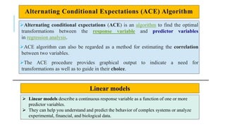
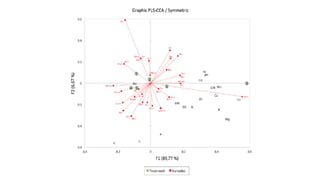
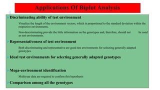
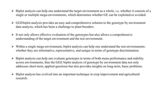
1. ADVANCED BIOMETRICAL AND
QUANTITATIVE GENETICS
UNIT-III

2. VASANTRAO NAIK MARATHWADA KRISHI
VIDYAPEETH, PARBHANI
COLLEGE OF AGRICULTURE, PARBHANI
Department:- Agricultural Botany
UNIT-III
Guided by:-
Dr. Jaghirdar
HOD
Department of Agril. Botany
Presented by:-
Akshay Deshmukh
Ph.D Scholar
2019 A/05P

3. INDEX
1
•Additive and Multiplicative Model
2
•Shifted Multiplicative Model
3
•Analysis and Selection of Genotype
4
•Methods and steps to select the best model
5
•Bioplot and mapping genotype

4. Alternating Conditional Expectations (ACE) Algorithm
Alternating conditional expectations (ACE) is an algorithm to find the optimal
transformations between the response variable and predictor variables
in regression analysis.
ACE algorithm can also be regarded as a method for estimating the correlation
between two variables.
The ACE procedure provides graphical output to indicate a need for
transformations as well as to guide in their choice.
Linear models
 Linear models describe a continuous response variable as a function of one or more
predictor variables.
 They can help you understand and predict the behavior of complex systems or analyze
experimental, financial, and biological data.

5. Nonparametric Regression
Nonparametric regression is a category of regression analysis in which the
predictor does not take a predetermined form but is constructed according
to information derived from the data.
Multicollinearity
refers to a situation in which two or more explanatory variables in a multiple
regression model are highly linearly related.
Multicollinearity exists whenever an independent variable is highly correlated with
one or more of the other independent variables in a multiple regression equation.
Multicollinearity is a problem because it undermines the statistical significance of an
independent variable.

6. ADDITIVE MODEL
It was suggested by Jerome H. Friedman and Werner Stuetzle (1981)
In statistics, an additive model (AM) is a nonparametric regression method.
It is an essential part of the ACE algorithm.
The AM uses a one-dimensional smoother to build a restricted class of
nonparametric regression models.
Because of this, it is less affected by the curse of dimensionality
e.g. a p-dimensional smoother.
The AM is more flexible than a standard linear model, while being more
interpretable than a general regression surface at the cost of approximation
errors.
Problems with AM include model selection, overfitting, and
multicollinearity.

7. MULTIPLICATIVE MODEL
Fisher and MacKenzie (1923) who used a multiplicative model to analyse a factorial arrangement
of 12 potato (Solarium tuberosum L) varieties.
 Applications of multiplicative models to the analysis of agricultural experiments involving different
cultivars of a crop species.
Finlay and Wilkinson (1963) and Eberhart and Russell (1966) introduced "stability analysis" that
uses a model in which the data on each cultivar is regressed on an environmental productivity index,
estimated as the main effect of the environment,
Thus introducing a term into the model which is multiplicative, i.e., the product of a cultivar
regression coefficient times an environment parameter, both of which are estimated from the data.
With the exception of estimation of variance components due to deviations of the cultivar yields
from their regressions, analysis using this model had previously been developed by Mandel (1961) to
provide a more general test for interaction in unreplicated two-way tables than Tukey's (1949) test of
nonadditivity.

8. TUKEY'S TEST
In statistics, Tukey's test of additivity, named for John Tukey, is an approach
used in two-way ANOVA (regression analysis involving two qualitative
factors) to assess whether the factor variables (categorical variables) are
additively related to the expected value of the response variable.

9. 1. Completely Multiplicative Model (COMM):
2. Shifted Multiplicative Model (SHMM):
3. Genotypes (cultivars) Regression Model (GREG)
4. Sites (environments) Regression Model (SREG)
5. Additive Main Effects and Multiplicative Interaction Model
(AMMI):

10. Additive And Multiplicative Model
The combined effects must either be greater for synergistic or less
than for an antagonistic outcome.
The additive model measures risk differences while the
multiplicative model uses ratios to measure effects.
The additive model has been suggested to be a better fit for
predicting disease risk in a population while
A multiplicative model is more appropriate for disease etiology.

11. Shifted Multiplicative Model
GE interaction
Most of the economic traits in plant breeding are quantitative nature.
Phenotypes values of the Cultivar/Genotypes are the combination of genotype (G)
and environment (E) values, and their interactions (GE).
defined as the variation in relative performance of genotypes in different
environnemental conditions.
In Crop Improvement program, because it complicates identification and selection of
superior genotypes thereby reducing genetic progress.

12. • Genotype X environment interaction (GEI) is the variation caused by the
joint effects of genotype and environments.
• Distinction between cross over interactions (COI) and non cross over
interaction (NCOI) is failed due to GEI.
• Cross over interactions results in the rank change of genotypes over different
environments.
• GEI complicate identification of superior genotype for range of environment.
If GEI is high, breeding gain is smaller.
• The shifted multiplication model (SHMM) was used to analyze interaction
between and among genotypes, locations and years in multi-environment trial
(MET) data.

13. IMPORTANCE OF GEI
Range Broad genetic background Narrow genetic background
Wide range of distinct
environment
Low heritability due to GEI
and unreliable ranking of
genotypes across
environment
Maximizing genetic variation
among environments and
significant means between
testing environments
Uniform environments
Maximizing genetic
variation and significant
means between testing
genotypes
Useless
A crossover interaction (also referred to as ordinal nonindependence), exists when the ordering of the data
points corresponding to the levels of one independent variable depends on the level of the other independent
variable.
Non crossover interaction There is really only one situation possible in which an interaction is significant,
but the main effects are not

14. ANALYSIS OF VARIANCE (ANOVA)
Source d.f.
1. Genotype g-1
2. Site s-1
3. Genotype X Site (g-1)(s-1)
4. Pooled error S(r-1)(g-1)
SHMM
5. Primary effects
6. Secondary effects
7. Tertiary effects

15. TYPES OF G X E
Interaction may be due to
1. Heterogeneity of genotypic variance across environments.
2. Imperfect correlation of genotypic performance across
environment

16.  Shifted multiplicative model was developed by Cornelius and
Seyedsadr in 1992
 SHMM is used to analyze the
complete separability,
genotypic separability,
environmental separability,
inseparability of environment effects and genotypic effects.
 Gregorius and Namkoong (1986) defined separability as the property
which is that cultivar effect is separable from environmental effect so
that there is no rank.

17. Genotypic
Separability
Complete
Separability
C

18. environmental
Separability
Inseparability

19. Cornelius et al. (1992) defined sufficient conditions for the absence of
statistically significant:
(1) SHMM1 is an adequate model for fitting the data.
(2) Primary effects of environments have the same sign. Non-significant
environmental rank-change interactions.
(3) Primary effects of genotypes have the same sign. The absence of
significance of both environmental rank change interactions.
Genotypic rank-change interactions occurs when (1), (2) and (3) all
hold.

20. Importance of SHMM
Categorization of location with similar environments helps breeders to
efficiently utilize resources and effectively target germplasm.
Useful tool to breeder in making decision on release of cultivar.
It helps in selection, testing and identifying superior genotypes.
Subsets of environment facilitate represent similar selection environment
facilitate the exchange of germplasm.

21. Methods And Steps To Select The Best Model
Several variance-covariance structures are available and were discussed in Hu
and Spilke (2011) in more detail.
Two main criteria to consider
First criterion
Akaike Information Criterion
(AIC) = -2LL + 2 x q
Where: LL denotes the log maximum likelihood of the related model.
q is the number of parameters of the variance-covariance structure.
Result of Criterion :- The model with the lower value of the information
criterion is preferred.

22. Second Criterion
• Schwarz Bayesian Information Criterion
(BIC or SIC) = -2LL + log(N) × q
• Where: LL denotes the log maximum likelihood of the related model
N is the total number of observations.
q is the number of parameters in the variance-covariance matrix.
• Result of Criterion :- The best model is again the model with the lower
value of the information criterion.
• The model with the smallest AIC and BIC in the METs is the best model.

23. Bioplot And Mapping Genotype
A biplot analysis is a scatter plot that approximates and graphically displays a two way
table by both its row and column factors such that relationships among the row factors,
relationships among the column factors, and the underlying interactions between the
row and column factors can be visualized simultaneously.
Biplot analysis is equivalent to principle component analysis (PCA).
While both biplot analysis and PCA use singular value decomposition as a key
mathematical technique.
Biplot analysis is a fuller use of SVD (singular value decomposition) to allow two
interacting factors to be visualized simultaneously.

24. PRINCIPLES OF BIPLOT ANALYSIS
Mathematically, a biplot may be regarded as a graphical display of matrix multiplication.
Given a matrix G with m rows and r columns, and a matrix R with r rows and n columns, they can be
multiplied to give a third matrix P with m rows and n columns.
If r=2, then matrix G can be displayed as the abscissa (x axis) and 2nd column the ordinate (y-axis).
Similarly, matrix E can be displayed as n points in a 2-D plot, with the 1st row as the abscissa and 2nd row
the ordinate.
A 2-D biplot is formed if the two plots are superimposed, which would contain m + n points.
An interesting property of this biplot is that it not only displays the m x n values of matrix p, because each
element of P can be visualized as :
Pij = xi x’j + yi y’j =giej = IgiIIgjIcosƟij
This equation is considered as the inner-product property of the biplot
where,
(xi,yi) – are the coordinates for row i and
(x’j, y’j) – are coordinates for column j
IgiI- is the vector length for row i
IejI – is the vector length for column j
Ɵij – is the angle between the vectors of row I and column j.

26. Applications Of Biplot Analysis
Discriminating ability of test environment
Visualize the length of the environment vectors, which is proportional to the standard deviation within the
respective environments.
Non-descriminating provide the little information on the genotypes and, therefore, should not be used
as test environments.
Representativeness of test environment
Both discriminating and representative are good test environments for selecting generally adapted
genotypes.
Ideal test environments for selecting generally adapted genotypes
Mega-environment identification
Multiyear data are required to confirm this hypothesis
Comparison among all the genotypes

27.  Biplot analysis can help one understand the target environment as a whole, i.e. whether it consists of a
single or multiple mega-environments, which determines whether GE can be exploited or avoided.
 GGEbiplot analysis provides an easy and comprehensive solution to the genotype by environment
data analysis, which has been a challenge to plant breeders.
 It not only allows effective evaluation of the genotypes but also allows a comprehensive
understanding of the target environment and the test environment.
 Within a single mega-environment, biplot analysis can help one understand the test environments:
whether they are informative, representative, and unique in terms of genotype discrimination.
 Biplot analysis can help one evaluate genotypes in terms of both mean performance and stability
across environments, thus the GGE biplot analysis of genotype by environment data not only
addresses short-term, applied questions but also provides insights on long-term, basic problems.
 Biplot analysis has evolved into an important technique in crop improvement and agricultural
research.

28. Thank
You