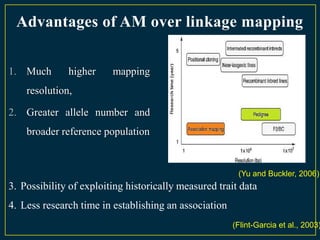
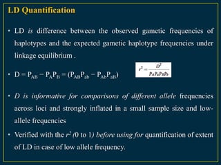
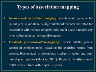
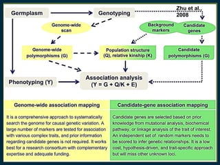
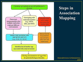
The document discusses advanced methods in crop improvement, focusing on the genetic basis of economically important traits and techniques for mapping quantitative trait loci (QTLs). It compares association mapping (AM) and linkage mapping, highlighting AM's advantages such as higher resolution and broader allele diversity. The text also describes specific software tools and approaches used for detecting associations between genotypes and phenotypes in various plant species.

1. • Hifzur Rahman

2. Methods in Crop Improvement
• To meet the food needs of the human population, plant breeders
select for agronomically important trais like yield.
• Determining the genetic basis of economically important complex
traits is a major goal.
• Linkage mapping has been a key tool for identifying the genetic
basis of quantitative traits in plants.
• Identification of QTLs or genes associated to particular trait
accelerated the pace of crop improvement either by introgressing
the identified QTLs/genes in desired genotype by MAB or by
transgenic technology.

3. QTL approach
 Uses standard bi-parental mapping populations
 F2 or RILs
 These have a limited number of recombination events.
 Resulting in low resolution of map i.e. the QTL covers many cM.
 Additional steps required to narrow QTL or clone gene.
 Difficult to discover closely linked markers for the causative gene

4. Association mapping (AM)
• Association mapping, also known as "linkage disequilibrium
mapping", is a method of mapping quantitative trait loci (QTLs) that
takes advantage of linkage disequilibrium to link phenotypes to
genotypes.
• Uses the diverse lines from the natural populations or germplasm
collections.
• Discovers linked markers associated (=linked) to gene controlling
the trait.

5. • Association studies are based on the assumption that a marker locus
is „sufficiently close‟ to a trait locus so that some marker allele
would be „travelling‟ along with the trait allele through many
generations during recombination. Murillo and Greenberg, 2008.
Major goal
• To identify inter-individual genetic variants, mostly single
nucleotide polymorphisms (SNPs), which show the strongest
association with the phenotype of interest, either because they are
causal or, more likely, statistically correlated or in linkage
disequilibrium (LD) with an unobserved causal variant(s).

7. Advantages of AM over linkage mapping
1. Much higher mapping
resolution,
2. Greater allele number and
broader reference population
(Yu and Buckler, 2006)
3. Possibility of exploiting historically measured trait data
4. Less research time in establishing an association
(Flint-Garcia et al., 2003)

8. Association analysis
Two approaches:-
 On the basis of distance between two loci
 By analyzing linkage disequilibrium between marker and target
gene in natural population.
• LD refers to nonrandom association of alleles at different loci.
• LD can occur between more distant sites or sites located in
different chromosomes

9. LD Quantification
• LD is difference between the observed gametic frequencies of
haplotypes and the expected gametic haplotype frequencies under
linkage equilibrium .
• D = PAB − PAPB = (PABPab − PAbPaB)
• D is informative for comparisons of different allele frequencies
across loci and strongly inflated in a small sample size and low-
allele frequencies
• Verified with the r2 (0 to 1) before using for quantification of extent
of LD in case of low allele frequency.

10. Calculation and visualization of LD:
• LD can be calculated using available haplotyping algorithms
• Maximum likelihood estimate (MLE).
• Pairwise LD can be depicted as a color-code triangle plot based on
significant pairwise LD level (r2, and D)
Computer softwares:
• “Graphical Overview of Linkage Disequilibrium” (GOLD )
• “Trait Analysis by aSSociation, Evolution and Linkage”
(TASSEL)
• PowerMarker

11. Factors affecting LD
 LD increases due to mating system (self-pollination), genetic
isolation, population structure, relatedness (kinship), small
founder population size or genetic drift, admixture, selection
(natural, artificial, and balancing), epistasis, and genomic
rearrangements.
 While factors like outcrossing, high recombination rate, high
mutation rate, gene conversion, etc., lead to a decrease/disruption
in LD.

12. LD Decay:
 LD will tend to decay with genetic
distance between the loci under
consideration.
 Loci attains linkage equilibrium (LE), i.e.
alleles are not preferentially paired
anymore.
 LD decays by one-half with each
generation of random mating.
 Thus, LD declines as the number of
generations increases, so that in old
populations LD is limited to small
distances. Raveendran et. al., 2008

13. Types of association mapping
1. Genome wide association mapping: search whole genome for
causal genetic variation. A large number of markers are tested for
association with various complex traits and it doesn‟t require any
prior information on the candidate genes.
2. Candidate gene association mapping: dissect out the genetic
control of complex traits, based on the available results from
genetic, biochemical, or physiology studies in model and non-
model plant species (Mackay, 2001). Requires identification of
SNPs between lines within specific genes.

14. Zhu et al.,
2008

15. Steps in
Association
Mapping
Abdurakhmonov & Abdukarimov,
2008

16.  Power to detect associations depends on
Sample size and experimental design
accurate phenotypic evaluations.
genotyping,
genetic architecture.

17. Phenotyping and Germplasm selection
Phenotyping
• Replications across multiple years in randomized plots and multiple
locations and environments
• influence of flowering time on other correlated traits, photoperiod
sensitivity, lodging, and susceptibility to prevalent pathogens because
these traits affect the measurement of other morphological or agronomic
traits at field condition. (Raveendran et al. 2008)
• Field Design:- incomplete block design (Lattice) (Eskridge, 2003).
Should be done on the basis of
• Diversity:- on the basis of phenotype and genotype
• Population structure

18. Germplasm selection and Population structure
• Randomly or non-randomly mated germplasm
• Randomly mated populations represent a rather narrow group of
germplasm, likely to lower resolution and harbor only a narrow
range of alleles
• Nonrandomly mated germplasm is used, population structure needs
to be controlled in the statistical analyses
(Yu et al., 2006)

19. • A set of unlinked, selectively neutral background markers are used
to achieve genome-wide coverage to broadly characterize the
genetic composition of individuals.
• Cluster analysis and boot strapping is done.
• On the basis of cluster analysis most diverse individuals are
selected from each cluster to represent the individuals of that
cluster.
• Helps in preventing spurious associations if population structure
and relatedness exist.

20. Rafalski et al 2010

21. Estimation of population structure
Low--dimensional projection
PCA based methods (Patterson et al., 2006)
Clustering
 Distance--based (Bowcock et al., 1994)
 Model--based
 STRUCTURE (Pritchard et al., 2000)
 mStruct (Shringarpure & Xing, 2008)

22. Evaluation of linkage disequilibrium and
associating genotype- phenotype
• Structure of linkage disequilibrium (LD) for a specific locus will,
reveal the association resolution possible at that locus.
• TASSEL (http://www.maizegenetics.net) is used to measure the
extent of LD as squared allele frequency correlation estimates (R2,
Weir, 1996) and measure the significance of R2.
• Eg. if LD decays within 1000 bp, then 1 or 2 markers per 1000 bp
will be needed to identify associations.
• Besides TASSEL there are many other softwares like DnaSP,
Arlequin etc. used to calculate D‟ and R2.

23. Softwares used in AM
Software Focus Description
Haploview 4.2 Haplotype LD and haplotype block analysis, haplotype population frequency estimation,
analysis and single SNP and haplotype association tests, permutation testing for
LD association significance
SVS 7 Stratification, Estimate stratification, LD, haplotypes blocks and multiple AM approaches for
LD and AM up to 1.8 million SNPs and 10,000 sample
TASSEL Stratification, LD and AM SSR markers, GLM and MLM methods
GenStat Stratification, LD and AM SSR markers, GLM and MLM-PCA methods
JMP genomics Stratification, LD and structured SNPs, CG and GWAS, analysis of common and rare Variants
AM
GenAMap Stratification, LD and structured SNPs, tree of functional branches, multiple visualization tools
AM
PLINK Stratification, LD and structured SNPs, multiple AM approaches, IBD and IBS Analyses
AM
STRUCTURE Population Compute a MCMC Bayesian analysis to estimate the proportion of the
structure genome of
an individual originating from the different inferred Populations
SPAGeDi Relative kinship genetic relationship analysis
BAPS 5.0 Population Compute Bayesian analysis to estimate the proportion of the genome of an
structure individual
and assign individuals to genetic clusters by either considering them as
immigrants or as descendents from immigrants
mStruct Population Structure Detection of population structure in the presence of admixing and mutations
from multi-locus genotype data. It is an admixture model which incorporates a
mutation process on the observed genetic markers
LDheatmap LD LD estimation (r2) displayed as heatmap plots using SNPs

24. Examples of association mapping studies
• Much of the association mapping in crop plants is just emerging from the
research phase and is beginning to be applied, especially in commercial
breeding setting.
• First attempt on candidate-gene association mapping study in plants
(maize) resulted in the identification of DNA sequence polymorphisms
within the D8 locus associated with flowering time (Thornsberry et al.,
2001).
• Using same population, Whitt et al., 2002 associated the candidate gene
su1 with sweetness taste , bt2, sh1 and sh2 with kernel composition, and
Wilson et al., 2004 ae1 and sh2 with starch pasting properties.

25. Association mapping studies in plant species

26. Association mapping studies in Rice
Population Sampl BG markers Trait Reference
e Size
Diverse land races 577 577 Starch quality (Bao et al., 2006)
Diverse accessions 103 123 SSRs Yield and its components (Agrama et al., 2007)
Landraces SSRs Heading date, plant height and Wen et al. (2009)
panicle length
Landraces SNPs Multiple agronomic traits Huang et al. (2010)
Diverse accessions 203 154 Trait of Harvest Index Li et al. (2012)
SSRs,1indel
Diverse accessions 210 86 SSRs yield and grain quality Borba et al. (2010)
diverse rice 383 44,000SNPs Aluminum Tolerance Famoso et al (2011)
accessions
Mini core 90 108 SSR+indel stigma and spikelet Yan et al. (2009)
collection characteristics
Diverse accessions 950 Sequence based Flowering time and grain yield Huang et al. (2011)
Diverse accessions 127 Sequence based Aroma Singh et al. (2010)
Diverse accessions 413 44K SNP chip Agronoical traits Zhao et al. (2011)

27. • Out of 18,000 accession of global origin, a USDA rice mini core
collection of 203 accession were used for phenotyping 14
agronomic traits.
• Out of 14 agronomic trait 5 traits were correlated with grain yield
per plant: plant height, plant weight, tillers, panicle length, and
kernels/ branch.
• Genotyped with 155 SSRs and Model based clustering using
STRUCTURE seperated the accessions into 5 main clusters
namely in ARO, AUS, TRJ,TEJ, IND.

28.  4 main groups (AUS, IND, TEJ and TRJ) were separately analyzed for the LD
measured by R2
 mean R2 ranged from 0.04 for IND to 0.10 for TEJ and TRJ.
 IND had the most linked marker pairs with significant LD (9.53%), while TRJ
had the least (5.57%).
 LD decay in distances was about 20 cM within both AUS and IND, while it
decayed about 30 and 40 cM within TRJ and TEJ

30. Association analysis on candidate genes
Association study employs techniques from molecular biology, field
sampling/breeding, bioinformatics and statistics.
1. Select candidate genes using existing QTL and positional cloning
2. Choose diverse germplasm for the trait.
3. Score phenotypic traits in replicated trials.
4. Amplify and sequence candidate genes.
5. Manipulate sequence into valid alignments and identify.
6. Obtain diversity estimates and evaluate patterns of selection
7. Statistically evaluate associations between genotypes and
phenotypes taking population structure into account.

32.  BADH gene was isolated from all 16 varieties and sequenced
 Sequence trace files from each variety were assembled into contigs
using combined Phred/Pharp/Consed software.
 Polymorphism tags were generated automatically by Polyphred
software integrated with the Consed.
 High quality SNPs from transcribed region were then identified
manually and screen shots of the SNP trace files for the two alleles.

33.  MassARRAY Assay Design 3.1software was further used to
detect more SNPs
 127 diverse rice varieties and landraces were used to analyse
polymorphism for the identified SNPs
 Phylogenetic tree of the BADH1 gene sequence obtained by
resequencing of 16 rice varieties and Nipponbare reference gene
sequence was constructed using MEGA 4.0.
 Analysis of the BADH1 sequence variation among 127 rice
varieties was done based on the scores of 15 validated SNPs
identified by resequencing of the BADH1 gene from 16 varieties
and Nipponbare using the Sequenom MassARRAY assays.

34. • Two common BADH1 protein haplotypes (corresponding to four
BADH1 SNP haplotypes) were analyzed in all 127 rice varieties
and also separately in the aromatic and salt-tolerant subgroups of
varieties
• 54 SNPs giving more than 95%success rates were used for the
population structure analysis using STRUCTURE software .
• Two haplotypes of the BADH1 protein, PH1 and PH2 were
modeled and docked.

35. • The three exonic SNPs were
• (1) S6 in exon 4 with a T/A polymorphism resulting in asparagine
to lysine substitution at amino acid position 144;
• (2) S18in exon 11 with a C/A polymorphism resulting in glutamine
to lysine substitution at amino acid position 345, and
• (3) S19 in exon 11 with T/C polymorphism resulting in isolucine to
threonine substitution at amino acid position 347.
• PH1 has 15 active GABald binding site where as PH2 has 8.

36. • 517 landraces were phenotyped and genotyped by sequencing upto
one fold coverage using Illumina Genome Analyzer II
• Aligned sequence reads to the rice reference genome for SNP
identification
• Discrepancies with rice reference genome were called as candidate
SNPs.

37. • A total of 3,625,200 nonredundant SNPs were identified, resulting
in an average of 9.32 SNPs per kb, with 87.9% of the SNPs located
within 0.2 kb of the nearest SNP
• A total of 167,514 SNPs were found in the coding regions of
25,409 annotated genes.
• 3,625 large-effect SNPs (representing mutations predicted to cause
large effects) were identified.
• Neighbor-joining tree as well as the
principal-component analysis
seperated rice germaplasm in two
groups i.e. indica and japonica.
• Further both indica and japonica had three subgroups.

38.  Genome-wide LD decay rates of indica and
japonica were estimated at ~123 kb and ~167
kb, where the r2 drops to 0.25 and 0.28,
 Because of strong population differentiation between the two
subspecies of cultivated rice GWAS was conducted only for 373
indica lines using mixed linear model (MLM)
 80 associations for the 14 agronomic traits were identified.
 Heading date strongly correlated with both population structure
and geographic distribution.

40. • 413 diverse accessions of O. sativa were phenotyped for 34
traits and genotyped using 44K SNP array.
• Probe was prepared from DNA, labelled and hybridized
against array.
• Genotype calling was done using ALCHEMY program
• 36,901 high-performing SNPs (call rate > 70 %) were used for all
analyses.

41. • PCA analysis was done to determine population structure and
separated all the accessions into 5 clusters.
• mixed model approach was implemented to correct population
structure
• SNP LD among the 44K common SNPs were detected using r2
using PLINK software.
• LD decay was observed at ~ 100 kb in indica ,
200 kb in aus and temperate japonica , and 300
kb in tropical japonica giving and average
marker distance of about 10kb

42. Plant Panicle length
height
Flowering time
Photoperiod
sensitivity

44. Comparison
Candidate gene Genome wide association Mapping
approach
GWA using Markers SNP genotyping Whole genome
using Microarray sequencing
• Choice of • Discovery of large • Good and robust • Detects all
candidate gene number of markers. can process large polymorphisms in
and marker number of sample the population
within them • In crops like A. and identify large thus avoids the
often involves thaliana (125Mb) no. of SNPs in erosion of power
some guess work ~140,000 and in one shot. due to
so chances are maize ascertainment
there many (475Mb)~10-15 • But if bias.
earlier million markers polymorphism is
unreported genes will be required to not present in
will go give complete initial discovery
undetected. coverage. panel remains
undetected in
large sample.