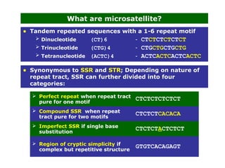
The document discusses molecular marker technologies and their applications in revealing genetic variation, emphasizing different types of molecular markers, such as microsatellites. It outlines various molecular techniques like PCR, electrophoresis, hybridization, and sequencing used to analyze genetic diversity, which is crucial for species' conservation. The document also explains the importance of genetic diversity for species' survival and resilience to diseases, presenting case studies and practical applications of these techniques.

1. MOLECULAR MARKER
TECHNOLOGIES

2. Outlines
 Organization and flow of genetic information
 Molecular techniques to reveal genetic variation
 Type of molecular markers
 Which marker for what purpose
 Microsatellite marker
 Case study 1: using microsatellites to estimate gene
flow via pollen
 Case study 2: using microsatellites for individual-
specific DNA fingerprints

3. FLOW OF GENETIC INFORMATION

4. DNA molecule consists of
two strands that wrap
around each other to
resemble a twisted ladder
A pairs with T
C pairs with G
Deoxyribonucleic Acid (DNA):
The molecule that encodes
genetic information

5. Nuclear DNA: Diploid; biparental inherited; recombination occur; can be viewed as a
huge ocean of largely nongenic DNA, with some tens of thousands of genes and gene
clusters scattered around like small islands and archipelagos. A high proportion of this
apparently nonfunctional DNA consists of repeated motifs and may be considered as
junk DNA or selfish DNA
Choroplast DNA: Haploid; usually maternally inherited in
angiosperms and paternally inherited in gymnosperms; typically ranging
from 135 to 160 kb in size, is packed with genes and thus resembles the
streamlined configuration of its cyanobacterial ancestral genome
Mitochondrial DNA: Haploid; typically maternally inherited; about 370 to 490
kb, about 10% of these sequences represent genes, another 10 to 26% were
found to be made up of repetitive DNA, including retrotransposons. Thus, the
majority of plant mtDNA sequences lack any obvious features of information

6. • Organism’s genomic DNAs are subjected to
mutation as a result of normal cellular operations or
interactions with environment
 Biology of organism
 Genomes under consideration
 Types of mutations
• The rates of mutation are depending on:

7. • Mutations in genomic DNA can be classified into
several categories:
GATCCGAGTGATCCGAGTAATCGCAATTAGCATCGCAATTAGCA
GATCCGAGTGATCCGAGTGGTCGCAATTAGCATCGCAATTAGCA
Base substitutionBase substitution
GATCCGAGTAGATCCGAGTATCGCATCGCAATTAGCAATTAGCA
GATCCGAGTAATTAGCAGATCCGAGTAATTAGCA
DeletionDeletion
GATCCGAGTATCGCAATTAGCAGATCCGAGTATCGCAATTAGCA
GATCCGAGTATCGCAGATCCGAGTATCGCAGCGCATTAGCAATTAGCA
InsertionInsertion
GATCCGAGTATCGCAATTAGCAGATCCGAGTATCGCAATTAGCA
GATCCGAGTATCGATCCGAGTATCTCTCGCGCAATTAGCAAATTAGCA
DuplicationDuplication
GATGATCCGCCGAGTATCGCAATTAGCAAGTATCGCAATTAGCA
GATGATGCCGCCAGTATCGCAATTAGCAAGTATCGCAATTAGCA
InversionInversion

8. Through long evolutionary accumulation, many
different instances of mutation as mentioned above
should exist in any given species
The number and degree of the various types of
mutations define the genetic diversity within a
species
It has been widely recognized that loss of genetic
diversity is a major threat for the maintenance and
adaptive potential of species

9. • Example - if low genetic
diversity, when a virulent
form of a disease arises,
many individuals may be
susceptible and die
S S
SS
S
S
S
S
S
S
S S
SS
S
S
S
S
S
S
Low Genetic diversity
All die
R S
SS
S
R
S
S
R
S
R S
SS
S
R
S
S
R
S
High Genetic diversity
Partially resistant
• But as a result of natural
genetic diversity within
local plant populations,
there may be some
individuals that are at least
partially resistant and there
are able to survive and
thus perpetuate the species

10. • For many plant species, ex situ and in situ
conservation strategies have been developed to
safeguard the extant of genetic diversity
• To manage this genetic diversity effectively the
ability to identify genetic diversity is
indispensable
• In addition, for this variation to be useful, it must
be heritable and discernable; as recognizable
phenotypic variation or as genetic mutation
distinguishable through molecular marker
technologies

11. Subsequently,
mutation arises
genetic variation at
DNA will cause
variation at the protein
level
Protein
markers
Mutation
Mutation arises
genetic variation at
the DNA level
DNA
markers
A sequence of DNA or protein that can be screened
to reveal key attributes of its state or composition
and thus used to reveal genetic variation
Definition of molecular markers

12. • Four major molecular techniques are commonly
applied to reveal genetic variation. These are:
 Polymerase chain reaction (PCR)
 Electrophoresis
 Hybridization
 DNA sequencing

13. POLYMERASE CHAIN REACTION
PCR is a procedure used to amplify (make multiple copies of) a
specific sequence of DNA
The method was invented by Kary Banks Mullis in 1983, for
which he received the Nobel Prize in Chemistry ten years later
three temperature-controlled step

14. ELECTROPHORESISELECTROPHORESIS
Migration rate depend on electrica
The termThe term 'electrophoresis''electrophoresis' literally means "to carry withliterally means "to carry with
electricity"electricity"
Technique for separating the components of a mixture ofTechnique for separating the components of a mixture of
charged molecules (proteins, DNAs, or RNAs) in an electriccharged molecules (proteins, DNAs, or RNAs) in an electric
field within a gel or other supportfield within a gel or other support

15. HYBRIDIZATION
One of the most commonly used
nucleic acid hybridization techniques
is Southern blot hybridization
Southern blotting was named after
Edward M. Southern who developed
this procedure at Edinburgh
University in the 1975

16. SEQUENCING
The process of determining the order of the nucleotide bases
along a DNA strand is called sequencing
In 1977, 24 years after the discovery of the structure of DNA,
two separate methods for sequencing DNA were developed:
chain termination method and chemical degradation method
Chain elongation proceeds until, b
Principle: single-stranded DNA molecules that differ in length
by just a single nucleotide can be separated from one another
using PAGE

17. Recent detection techniques
TaqMan – a probe used to detect specific sequences in PCR
products by employing 5’ to 3’ exonuclease activity of the Taq
DNA polymerase
Microarray Technology – a high throughput screening
technique based on the hybridization between oligonucleotide
probes (genomic DNA or cDNA) and either DNA or mRNA
Pyrosequencing – refers to sequencing by synthesis, a simple
to use technique for accurate analysis of DNA sequences

18. TYPES OF MOLECULAR MARKERS
• Due to rapid developments in the field of molecular genetics, a
variety of molecular markers has emerged during the last few
decades
Biochemical
marker
Allozyme
Non-PCR based
marker
RFLP, Minisatellite (VNTR)
PCR based
marker
Microsatellite, RAPD, AFLP, CAPS
(PCR-RFLP), ISSR, SSCP, SCAR,
SNP, etc.
Traditional
marker systems
PCR generation:
in vitro DNA
amplification

19. Allozyme (biochemical marker)
Technique: Electrophoresis and enzyme
staining
• The alternative forms of a particular protein visualized on a gel
as bands of different mobility. Polymorphism due to mutation
an amino acid has been replaced, the net electric charge of the
protein may have been altered

20. RFLP (Non-PCR based marker)
Techniques: Electrophoresis and
hybridization
• Targets variation in DNA restriction sites and in DNA restriction
fragments. Sequence variation affecting the occurrence (absence
or presence) of endonuclease recognition sites is considered to
be main cause of length polymorphisms

21. RAPD (PCR-based marker)
Techniques: PCR and
Electrophoresis
Uses primers of random sequence to amplify DNA fragments by
PCR. Polymorphisms are considered to be primarily due to variation
in the primer annealing sites, but they can also be generated by
length differences in the amplified sequence between primer
annealing sites

22. AFLP (PCR-based marker)
Techniques: PCR and Electrophoresis
• A variant of RAPD. Following restriction enzyme digestion of DNA,
a subset of DNA fragments is selected for PCR amplification and
visualization

23. Peak: Scan 3512 Size 143.84 Height 158 Area 1485
142 144 146 148 150 152 154 156 158 160 162 164 166 168 170 172 174 176 178 180 182 184
12_08.f sa 8 Green
1000
2000
3000
155.02 163.13
13_10.f sa 10 Green
1000
2000
3000
4000
155.06 161.09
14_12.f sa 12 Green
1000
2000
3000
4000
154.98 161.01
15_14.f sa 14 Green
1000
2000
153.01 157.03
16_16.f sa 16 Green
1000
2000
3000
155.10 157.05
17_01.f sa 1 Green
2000
4000
155.06 163.09
18_03.f sa 3 Green
2000
4000
156.13 165.12
Microsatellite (PCR based marker)
Techniques: PCR and
Electrophoresis
• Targets tandem repeats of a small (1-6 base pairs) nucleotide
repeat motif. Polymorphism due to the number of tandem
repeats

24. Other markers
• Cleaved Amplified Polymorphic Sequence (CAPS/PCR-RFLP)
• Inter Simple Sequence Repeat (ISSR)
• Single-strand conformation Polymorphism (SSCP)
• Sequence Characterized Amplified Region (SCAR)
More recent markers
• Single-Nucleotide Polymorphism (SNP)
• Retrotransposon-based markers
 Sequence-Specific Amplified Polymorphism (S-SAP)
 Inter-retrotransposon Amplified Polymorphism (IRAP)
 Retrotransposon-Microsatellite Amplified Polymorphism (REMAP)
 Retrotransposon-Based Insertional Polymorphism (RBIP)

25. Weising, K., Nybom, H., Wolff, K. and Kahl, G. 2005. DNA
Fingerprinting in Plants, Priciples, Methos, and Applications. 2nd
Edition. CRC Press, Boca Raton, Florida, USA.
Spooner, D., van Treuren, R. and de Vicente, M.C. 2005.
Molecular markers for genebank management. IPGRI Technical
Bulletin No. 10. International Plant Genetic Resources Institute,
Rome, Italy.
Henry, R.J. 2001. Plant Genotyping: The DNA Fingerprinting of
Plants. CAB International Publishing, Wallingford, U.K.

26. Markers differ with respect to important
features:
• Genomic abundance
• Polymorphism level
• Locus specificity
• Reproducibility
• Technical requirements
• Financial investment

27. • Codominance or dominace
Dominant marker:
A marker shows dominant inheritance with
homozygous dominant individuals
indistinguishable from heterozygous
individuals
Codominant marker:
A marker in which both alleles are
expressed, thus heterozygous individuals
can be distinguished from either
homozygous state

28. None of the available techniques is superior to all others for a
wide range of applications, but the key-question rather is
which marker to use in which situation
.
• Within and among population variation – Allozyme, SSR, AFLP and RAPD
• Genetic Linkage Mapping – AFLP, RAPD, Allozyme, RFLP, SSR, CAPS, SNP
• Mating system study – Allozyme or microsatellite
• Estimating gene flow via pollen and seed – Microsatellite (SSR)
• Phylogeography – cpSSR
• Clonal identification – AFLP or RAPD
• Polyploidy – multilocus dominant marker (AFLP)
• Phlogenetic study – conserve within species (DNA sequencing)
Intraspecific (among individuals) – markers target less conserve region
Interspecific (among species) – markers target more conserve region

29. • A framework for selecting appropriate
techniques for plant genetic resources
conservation can be referred to:
Karp, A., Kresovich, B., Bhat, K.V., Ayad, W.G. and Hodgkin, T.
1997. Molecular Tools in Plant Genetic Resources Conservation: A
Guide to the Technologies. IPGRI Technical Bulletin No. 2.
International Plant Genetic Resources Institute, Rome, Italy

30. Microsatellite marker
 What are microsatellite?
 Where are microsatellites found?
 How do microsatellites mutate?
 Abundance in genome
 Why do microsatellite exist?
 Models of mutation
 Development of microsatellite primers
 Genotyping procedure
 Advantages
 Disadvantages
 Applications

31. What are microsatellite?
• Tandem repeated sequences with a 1-6 repeat motif
 Dinucleotide (CT)6 - CTCTCTCTCTCT
 Trinucleotide (CTG)4 - CTGCTGCTGCTG
 Tetranucleotide (ACTC)4 - ACTCACTCACTCACTC
• Synonymous to SSR and STR; Depending on nature of
repeat tract, SSR can further divided into four
categories:
 Perfect repeat when repeat tract
pure for one motif
CTCTCTCTCTCT
 Compound SSR when repeat
tract pure for two motifs
CTCTCTCACACA
 Imperfect SSR if single base
substitution
CTCTCTACTCTCT
 Region of cryptic simplicity if
complex but repetitive structure
GTGTCACAGAGT

32. Where are microsatellites found?
Majority are in non-coding region

33. How do microsatellites mutate?
DNA polymerase slippage Unequal crossing over
• Microsatellites alleles change rather quickly over time
 E. coli – 10-2
events per locus per replication
 Drosophila – 6 X 10-6
events per locus per generation
 Human – 10-3
events per locus per generation

34. Abundance in genome
• Microsatellites have been found in every organism
studied so far
• Most frequent in human > insect > plant > yeast >
nematode
GA/CT Dipterocarp
GA/CT & CA/GT Conifer
• Most common dinucleotide:
CA/GT Human

35. Why do microsatellite exist?
• Majority are found in non-coding regions; thought
no selective pressure; as "junk" DNA?
• In plant, high density of SSRs were found in close
proximity to coding regions; regulatory properties
• Regulate gene expression and protein function,
e.g., human diseases caused by expansions of
polymorphic trinucleotide repeats in genes fragile X
and myotonic dystrophy
• High level of polymorphism; a necessary source of
genetic variation

36. Models of Mutation
• Size matters when doing statistical tests of population
substructuring
• The mutation model still unclear but stepwise mutation
appears to be the dominant force creating new alleles in
the few model organisms studied to date
 Stepwise Mutation Model (SMM) - when SSRs mutate,
they gain or lose only one repeat
 Two alleles differ by one repeat are more closely
related than alleles differ by many repeats
CTCTCT
CTCTCTCT
CTCTCTCTCT
CTCTCT
CTCTCTCT
CTCTCTCTCT
• Several statistics based on estimates of allele frequencies
(e.g., Fst & Rst) rely explicitly on a mutation model

37. Development of microsatellite primers
• Standard method to isolate microsatellites from clones
 Creation of a small insert genomic library
 Library screening by hybridization
 DNA sequencing of positive clones
 Primer design and PCR analysis
 Identification of polymorphisms
• Can be time consuming and expensive. May be
obtained by screening sequence in databases or
screening libraries of clones
• This approach can be extremely tedious and inefficient
for species with low microsatellite frequencies

38. • Alternative strategies to overcome
 Selective hybridization using nylon membrane
 Selective hybridization using steptavidin coated beads
 RAPD based
 Primer extension

39. Genotyping procedure
PCR
Electrophoresis
Agarose Denaturing PAGE CapillaryPAGE
Visualization
Silver
staining
SybrGreen
staining
Autoradio-
graphy
Fluorescent
dyes

40. • The use of fluorescently labeled primers, combine with
automated electrophoresis system greatly simplified
the analysis of microsatellite allele sizes
Primer1
Primer2
Primer4
Primer3
102 104 106 108 110 112 114 116 118 120 122 124 126 128 130 132 134 136 138 140 142 144 146 148 150
29_10.f sa 10 Green
2000
4000
6000
122.29
30_12.f sa 12 Green
1000
2000
3000
4000
119.09 122.28
31_14.f sa 14 Green
1000
2000
120.24 124.18
32_16.f sa 16 Green
1000
2000
3000
123.34 131.42
33_01.f sa 1 Green
1000
2000
120.23 126.40
34_03.f sa 3 Green
2000
4000
120.24 124.33
35_05.f sa 5 Green
1000
2000
120.24 122.29
Locus 1
Peak:Scan2946 Size106.67 Height108 Area775
92 94 96 98 100 102 104 106 108 110 112 114 116 118 120 122 124 126 128 130 132 134 136 138 14
017_01.f sa 1 Blue
107.62 111.87
018_03.f sa 3 Blue
109.75 116.16
019_05.f sa 5 Blue
107.69
020_07.f sa 7 Blue
109.78
021_09.f sa 9 Blue
109.78 111.88
022_11.f sa 11 Blue
109.69 118.45
023_13.f sa 13 Blue
103.36 107.59
Locus 2Peak:Scan3100 Size257.25 Height110 Area668
242 244 246 248 250 252 254 256 258 260 262 264 266 268 270 272 274 276 278 280 282 284 286 288 2901a.f sa 34 Blue
1000
2000
260.20
2a.f sa 26 Blue
1000
2000
260.20
261.18
3a.f sa 31 Blue
200
400
600
800
261.18
4a.f sa 20 Blue
300
600
900
260.20 266.10
5a.f sa 8 Blue
300
600
900
266.10
6a.f sa 35 Blue
500
1000
1500
2000
266.04
267.01
7a.f sa 36 Blue
500
1000
1500
267.06
Locus 3
Peak: Scan 1919 Size149.07 Height67 Area 309
132 134 136 138 140 142 144 146 148 150 152 154 156 158 160 162 164 166 168 170 172 174 176 178 180 182 184 186 188 19004b.f sa 10 Green
1000
2000
3000
150.93 155.07
05b.f sa 13 Green
1000
2000
3000
155.07 163.02
06b.f sa 16 Green
1000
2000
3000
155.02 163.02
07b.f sa 19 Green
1000
2000
3000
155.13 163.02
08b.f sa 22 Green
1000
2000
3000
4000
150.94 158.96
09b.f sa 2 Green
1000
2000
3000
4000
155.02 163.00
10b.f sa 5 Green
1000
2000
3000
4000
150.94 155.02
11b.f sa 8 Green
1000
2000
3000
4000
155.07
Locus 4

41. 106 108 110 112 114 116 118 120 122 124 126 128 130 132 134
01-068.fsa 7 Yellow
1000
2000
3000
118.36 120.50
121.41
02-052.fsa 7 Yellow
2000
4000
120.50 122.49
123.40
03-115.fsa 5 Yellow
500
1000
1500
2000
118.37 120.49
121.39
122.54
123.43
04-054.fsa 11 Yellow
500
1000
1500
120.50 124.53
05-022.fsa 11 Yellow
500
1000
1500
120.49 126.55
06-039.fsa 13 Yellow
500
1000
1500
2000
120.49 128.52
120/120
122/122
120/122
120/124
120/126
120/128
Extra A
Non-templated addition
of an extra A to 3’ end of
PCR products
Stutter
Numberous bands differ in
size by 2 bp caused by
slippage of DNA polymerase

42. 0 112 114 116 118 120 122 124 126 128 130 132 134 136 138 140 142 144 146 148 150
2000
4000
6000
122.29
1000
2000
3000
4000
119.09 122.28
1000
2000
120.24 124.18
1000
2000
3000
123.34 131.42
1000
2000
120.23 126.40
2000
4000
120.24 124.33
1000
2000
Peak: Scan 3034 Size 255.35 Height 193 Area 1214
236 238 240 242 244 246 248 250 252 254 256 258 260 262 264 266 268 270 272 274 276 278 280 282 284 286 288 290
09a.fsa 2Blue
2000
4000
6000
258.23 266.19
10a.fsa 5Blue
2000
4000
258.32 266.21
11a.fsa 8Blue
2000
4000
6000
258.23 266.19
12a.fsa 11Blue
2000
4000
253.31 266.19
13a.fsa 14Blue
2000
4000
6000
266.20
14a.fsa 17Blue
2000
4000
258.33 266.30
15a.fsa 20Blue
2000
4000
1000
150.93 155.07
05b.fsa 13Green
1000
2000
3000
155.07 163.02
06b.fsa 16Green
1000
2000
3000
155.02 163.02
07b.fsa 19Green
1000
2000
3000
155.13 163.02
08b.fsa 22Green
1000
2000
3000
4000
150.94 158.96
09b.fsa 2Green
1000
2000
3000
4000
155.02 163.00
10b.fsa 5Green
1000
2000
3000
4000
150.94 155.02
11b.fsa 8Green
1000
2000
3000
4000
86 88 90 92 94 96 98 100 102 104 106 108 110 112 114 116 118 120 122 124 126 128 130 132 134 136 138 140
15h_13.fsa 13Yellow
1000
2000
3000
107.17 109.23 111.40
16h_15.fsa 15Yellow
1000
2000
3000
4000
96.88 98.85 100.87
17h_02.fsa 2Yellow
2000
4000
107.11 109.24 111.30
18h_04.fsa 4Yellow
1000
2000
3000
4000
107.18 109.24 111.40
19h_06.fsa 6Yellow
2000
4000
98.83 100.80 102.92 117.69 119.82 121.85
20h_08.fsa 8Yellow
1000
2000
3000
107.15 109.23 111.32
183.66
185.63
189.56
191.53
195.38
197.35
12e_08.fsa 8Blue
100
200
13e_10.fsa 10Blue
100
200
300
14e_12.fsa 12Blue
100
200
15e_14.fsa 14Blue
50
100
150
200
16e_16.fsa 16Blue
200
400
600
17e_01.fsa 1Blue
300
600
900
18e_03.fsa 3Blue
200
400
600

43. Advantages
 Low quantities of template DNA required (10-100 ng)
 High genomic abundance
 Random distribution throughout the genome
 High level of polymorphism
 Band profiles can be interpreted in terms of loci and alleles
 Codominance of alleles
 Allele sizes can be determined with an accuracy of 1 bp,
allowing accurate comparison across different gels
 High reproducibility
 Different SSRs may be multiplexed in PCR or on gel
 Wide range of applications
 Amenable to automation

44. Disadvantages
 High development costs in case primers are not yet
available. Primers might be species specific
 Heterozygotes may be misclassified as homozygotes when
null-alleles occur due to mutation in the primer annealing
sites
 Stutter bands on gels may complicate accurate scoring of
polymorphisms
 Underlying mutation model (infinite alleles model or
stepwise mutation model) largely unknown
 Homoplasy due to different forward and backward
mutations may underestimate genetic divergence

45. Applications
 Population genetics: investigations within a genus of centers
of origin, genetic diversity, population structures and
relationships among species
 Parentage analysis: seed orchard monitoring, mating systems
and gene flow via pollen & seed
 Fingerprinting: clone confirmation and individual-specific
fingerprints
 Genome mapping - Constructing full coverage or QTL maps
 Comparative mapping - Genome structure, framework maps,
or transferring trait and marker data among species
Generally, high mutation rate makes them informative and
suitable for intraspecific studies but unsuitable for studies
involving higher taxonomic levels

46. Case study 1: Using
microsatellites to estimate
gene flow via pollen

47.  Effective breeding unit?
 Pollen flow distance?
 Outcrossing rate?

48. Shorea leprosula Shorea parvifolia

49. Methodology
Sample collection
DNA extraction
SSRs analysis
1. Gene flow: exclusion and likelihood approaches
2. Effective breeding unit: Nason et al. (1998)
3. Model of pollen dispersal to get maximum pollen
flow distance
SSRs development
Data analysis

50. No. of
clones
sequenced
No. of
clones with
SSR (%)
No. of
unique SSR
clones (%)
Core sequence (no. of clones; % &
repeat times)
624
592
(94.9)
315
(53.2)
CT/GA (266; 84.4 & 6-78)
GT/CA (29; 9.2 & 8-46)
Others (20; 6.4 & 6-40)
Microsatellite Loci
Locus
Primer sequence (5’
– 3’)
Repeat
motif
Length N
Size
range
He PIC
lep074a
F: ATC ACC AAG TAC CTA TCA TCA
R: GCA ATG GCA CAC AGT CTA TC (CT)11 124 11 110-130 0.824 0.791
lep079
F: GTT GTC TGT TCT TAC CAG GAA G
R: GCA TAA GTA TCG TCG CCA (CT)11 162 13 155-198 0.830 0.798
lep111a
F: GGA AAC TAC TGG AGC AGA GAC
R: GGT GGG TTA TGG AGA ATG AG (GA)14 152 12 138-154 0.855 0.821
lep118
F: AAA GCG TAC AAA TTC ATC A
R: CTA TTG GTT GGG TCA GAA GG (GA)16 170 15 145-176 0.892 0.861
lep280
F: GCA ACT AAA ATG GAC CAG A
R: GAG TAA GGT GGC AGA TAT AGA G (CT)7 119 11 107-137 0.851 0.816
lep384
F: CCA AGA CAA CTC AAT CCT CA
R: AGA TGA AGG TGT TGC TGT G (CT)13 206 14 191-219 0.657 0.632
lep562
F: TGA TTT GGG TGG TTG TAG
R: TAT TAC ATT TTT CAA GTC AAG TC (GT)8 164 12 154-180 0.883 0.852
Lee, S.L. et al. 2004. Isolation and characterization of 21 microsatellite loci in an important tropical tree
Shorea leprosula and their applicability to S. parvifolia. Molecular Ecology Notes 4: 222-225

51. 50 ha demographic plot in Pasoh Forest
Reserve

52. 0
100
200
300
400
500
0 100 200 300 400 500 600 700 800 900 1000
Distance/m
Distance/m
Pasoh Forest Reserve - 50-ha plot (190 individuals of S. leprosula and 102
of S. parvifolia ≥ 27 cm dbh within the 50-ha plot)

56. • Shorea leprosula – 9 loci (Pe = 0.999)
 lep074a, lep384, lep111a, lep118, lep280,
lep267, lep294, lep475 & lep562
 PCR (500 x 9 = 4500 reactions)
• Shorea parvifoila – 6 loci (Pe = 0.999)
 lep074a, lep384, lep111a, lep118, lep280 &
lep294
 PCR (360 x 6 = 2160 reactions)

57. 0
50
100
150
200
250
300
350
400
450
500
0 50 100 150 200 250 300 350 400 450 500 550 600 650 700 750 800 850 900 950 1000
S. leprosula (SL48)
MT4
8

58. 0
50
100
150
200
250
300
350
400
450
500
0 50 100 150 200 250 300 350 400 450 500 550 600 650 700 750 800 850 900 950 1000
MT3
5
S. parvifolia (SP35)

59. Mother tree
(no. of seed analyzed)
Mean distance
between MT
% outcrossing
(no. of seed)
% pollen
outside plot
Mean pollen flow
distance
Shorea leprosula
SL048 (45) 267.1 ± 136.2 93.3 (42) 20.0 (9) 152.9 ± 99.6
SL062 (44) 363.2 ± 151.6 88.6 (39) 20.5 (9) 302.6 ± 188.9
SL074 (48) 259.2 ± 151.2 85.4 (41) 18.8 (9) 148.6 ± 187.2
SL075 (43) 292.6 ± 145.8 67.4 (29) 18.6 (8) 173.1 ± 103.8
SL084 (46) 512.6 ± 228.3 82.6 (38) 23.9 (11) 448.2 ± 245.3
SL109 (45) 343.7 ± 158.8 95.6 (43) 33.3 (15) 285.0 ± 154.5
SL160 (44) 567.1 ± 243.1 81.8 (36) 31.8 (14) 580.3 ± 288.4
Mean 372.2 ± 121.6 85.0 ± 9.3 23.8 ± 6.2 298.7 ± 164.0
Shorea parvifolia
SP009 (32) 309.0 ± 166.5 59.4 (19) 9.4 (3) 61.9 ± 100.5
SP014 (48) 307.7 ± 165.1 62.5 (30) 14.6 (7) 105.1 ± 140.9
SP020 (42) 348.7 ± 172.2 85.6 (36) 33.3 (14) 194.0 ± 146.7
SP022 (47) 239.6 ± 133.2 72.3 (34) 21.3 (10) 148.2 ± 125.0
SP025 (46) 376.2 ± 192.4 56.5 (26) 19.6 (9) 317.1 ± 277.0
SP035 (44) 244.2 ± 139.9 22.7 (10) 2.3 (1) 185.0 ± 159.7
Mean 304.2 ± 54.7 59.8 ± 21.1 16.8 ± 10.7 168.6 ± 88.1

60. Mother tree
(no. of seed analyzed)
Breeding unit parameters
Size (individual) Area (ha) Radius (m)
Shorea leprosula
SL048 (45) 203.6 63.6 450.1
SL062 (44) 208.0 65.0 454.9
SL074 (48) 205.0 64.1 451.6
SL075 (43) 221.0 69.0 468.8
SL084 (46) 225.2 70.4 473.3
SL109 (45) 245.7 76.8 494.4
SL160 (44) 261.8 81.8 510.3
Mean 224.3 ± 22.1 70.1 ± 6.9 471.9 ± 23.0
Shorea parvifolia
SP009 (32) 81.9 59.4 434.7
SP014 (48) 90.0 65.2 455.6
SP020 (42) 112.9 81.8 510.3
SP022 (47) 97.8 70.8 474.8
SP025 (46) 105.5 76.5 493.4
SP035 (44) 76.7 55.6 420.5
Mean 94.1 ± 13.9 68.2 ± 10.1 464.9 ± 34.5

61. A:datapollen curve testing tembaga.xls
Rank 2 Eqn 8157 Exponential(a,b)
r^2=0.8084237 DF Adj r^2=0.78588531 FitStdErr=0.02007574 Fstat=75.957342
a=0.16445904
b=346.58324
0 200 400 600 800 1000
Distance
0
0.025
0.05
0.075
0.1
0.125
0.15
0.175
Frequency
0
0.025
0.05
0.075
0.1
0.125
0.15
0.175
Frequency
A:datapollen curve testing sarang.xls
Rank 29 Eqn 8157 Exponential(a,b)
r^2=0.81184414 DF Adj r^2=0.78289709 FitStdErr=0.046788411 Fstat=60.4064
a=1.3650821
b=42.410263
0 200 400 600 800
Distance
0
0.05
0.1
0.15
0.2
0.25
0.3
0.35
0.4
0.45
Frequency
0
0.05
0.1
0.15
0.2
0.25
0.3
0.35
0.4
0.45
Frequency
Negative exponential curve
y = ae(-x/c)

62.  Moderate pollen flow (150 – 300 m) – Thrips as
pollinators
 Predominant outcrossing (85%) & mix-mating (60%)
 Model for pollen dispersal – negative exponential model
 Optimum population size for conservation - breeding
unit area & breeding unit size obtained (about 70 ha)
Conclusion

63. Case study 2: Using
microsatellites for individual-
specific DNA fingerprints

64. In forensic applications in forestry and chain of custody
certification, two types of databases are required
To track the illegal log into
its original population
Required fingerprinting
databases for population
identification
To match the illegal log into
its original stump
Required fingerprinting
databases for individual
identification

65. DNA markers to match the illegal log into its original stump
Log being stolen / Illegal logging
Collect sample for DNA extraction
• Perform DNA analysis using DNA markers
• Comparison of DNA profiles of log & stump
• If the same, they are from the same tree
Stump being left behind
Collect sample for DNA extraction

66. • However, In DNA testimony, it is necessary to provide an
estimate of the weight of the evidence
• Three possible outcomes of a DNA test: no match,
inconclusive, or MATCH between samples examined
• If MATCH, it would not be scientifically justifiable to speak
of a match as poor proof of identity in the absence of
underlying data that permit some reasonable estimate of
how rare the matching characteristics actually are
• Therefore, in forensic casework, a population database
must be established for statistical evaluation of the
evidence to extrapolate the possibility of a random match
Random
MATCH!!

67. Neobalanocarpus heimii

68. Methodology
Sample collection
DNA extraction
SSRs analysis
Comprehensive DNA fingerprinting databases of N.
heimii generated for individual identification
throughout P. Malaysia
SSRs screening
Data analysis

69. BEn
Sun
Pia
Bub
Chi
Jel
GB
a
Leb
HTB
HTA
PRa
RD
a
Ter
RTu
Lak
BTi
Len Ke
m
Ber
Les
Gom
SLa
Amp
Pas
Pel
Lab LeB
LeA
PaA
PaB
KEDAH
Bkt. Enggang (BEn)
Sungkop (Sun)
PERAK
Piah (Pia)
Bubu (Bub)
Chikus (Chi)
SELANGOR
Sg Lalang (SLa)
Ampang (Amp)
Gombak (Gom)
N. SEMBILAN
Pasoh (Pas)
Pelangai (Pel)
JOHOR
Labis (Lab)
Panti C16 (PaA)
Panti C68 (PaB)
Lenggor C32 (LeA)
Lenggor C76 (LeB)
KELANTAN
Lebir (Leb)
Jeli (Jel)
G. Basor (GBa)
TERENGGANU
Rambai Daun (RDa)
H. Terengganu C31
(HTA)
H. Terengganu C14A
(HTB)
Pasir Raja (PRa)
PAHANG
Lesong (Les)
Bkt. Tinggi (BTi)
Rotan Tunggal (RTu)
Tersang (Ter)
Lentang (Len)
Lakum (Lak)
Kemasul (Kem)
Berkelah (Ber)
Sample collection

70. SSRs screening
51 SSR primer pairs developed for dipterocarps
• Neobalanocarpus heimii (6) (Iwata et al. 2000)
• Shorea lumutensis (2) (Lee et al. 2006)
• Shorea leprosula (21) (Lee et al. 2004a)
• Hopea bilitonensis (15) (Lee et al. 2004b)
• Shorea curtisii (7) (Ujino et al. 1998)

71. Specific amplification
Peak: Scan 1583 Size 118.12 Height 111 Area 616
106 108 110 112 114 116 118 120 122 124 126 128 130 132 134 136 138 140 142 144 146 148 150 152 154
24b.f sa 24 Blue
100
200
25b.f sa 25 Blue
20
40
60
26b.f sa 28 Blue
100
200
300
27b.f sa 31 Blue
20
40
60
80
28b.f sa 34 Blue
20
40
60
80
29b.f sa 25 Blue
50
100
30b.f sa 28 Blue
30
60
90
31b.f sa 31 Blue
20
40
60
80
32b.f sa 34 Blue
100
200
300
Peak: Scan 2946 Size 106.67 Height 108 Area 775
92 94 96 98 100 102 104 106 108 110 112 114 116 118 120 122 124 126 128 130 132 134 136 138 140
017_01.fsa 1 Blue
1000
2000
3000
107.62 111.87
018_03.fsa 3 Blue
1000
2000
109.75 116.16
019_05.fsa 5 Blue
1000
2000
3000
107.69
020_07.fsa 7 Blue
2000
4000
109.78
021_09.fsa 9 Blue
1000
2000
109.78 111.88
022_11.fsa 11 Blue
500
1000
1500
109.69 118.45
023_13.fsa 13 Blue
1000
2000
103.36 107.59

72. P e a k : S c a n 1 7 8 7 S i z e 1 4 4 . 7 9 H e i g h t 4 2 1 A r e a 2 0 3 8
122 124 126 128 130 132 134 136 138 140 142 144 146 148 150 152 154 156 158 160 162 164 166 168 170 172 174 176 178 18001a.f sa 1 Blue
200
400
146.83 150.89
02a.f sa 4 Blue
2000
4000
6000
146.71
03a.f sa 7 Blue
2000
4000
6000
146.83
04a.f sa 10 Blue
2000
4000
6000
150.77
05a.f sa 13 Blue
2000
4000
6000
146.81 150.88
06a.f sa 16 Blue
2000
4000
6000
150.77
07a.f sa 19 Blue
1000
2000
3000
146.81 150.88
Maternal genotype
Half-sib
genotypes
Qualitative observations (each progeny possessed at least one maternal
allele) to support the postulation of single-locus mode of inheritance
Mode of inheritance

73. Null allele
 Homozygote excess (MICROCHECKER; Van
Oosterhout et al. 2004)
 Examine patterns of inheritance
 If any Individuals repeatedly fail to amplify any
alleles at just one locus while other loci amplify
normally

74. H Shc09 (CT)n ? (A)n
Allele 186a GGAAAAAAAAAAAAAAAAAA........TACGTACTTTTCGTTTTAGTTACGTTTTTCAATACCAAGAGA 70
Allele 186b GGAAAAAAAAAAAAAAAAAA........TACGTACTTTTCGTTTTAGTTACGTTTTTCAATACCAAGAGA
Allele 186c GGAAAAAAAAAAAAAAAAAA........TACGTACTTTTCGTTTTAGTTACGTTTTTCAATACCAAGAGA
Allele 187 GGAAAAAAAAAAAAAAAAAAA.......TACGTACTTTTCGTTTTATTTACGTTTTTCAATACCAAGAGA
Allele 194 GGAAAAAAAAAAAAAAAAAAAAAAAAAATACGTACTTTTCGTTTTAGTTACGTTTTTCAATACTAAGAGA
G Sle605 (GA)n ? (GA)n(CA)n(GA)n
Allele 118a CCCGAGGAAGGGGGCAGAGAGACACAGAGAGAGAGAGAGA....GGCAGATGGAGGGAC.GGCGACAGCA 70
Allele 118b CCCGAGGAAGGGGGCAGAGAGACACAGAGAGAGAGAGAGA....GGCAGATGGAGGGAC.GGCGACAGCA
Allele 118c CCCGAGGAAGGGGGCAGAGAGACACAGAGAGAGAGAGAGA....GGCAGATGGAGGGAC.GGCGACAGCA
Allele 119 CCCGAGGAAGGGGGCAGAGAGACACAGAGAGAGAGAGAGA....GGCAGATGGAGGGACCAGCGACAGCA
Allele 121 CCCGAGGAAGGGGGCAGAGA..CACAGAGAGAGAGAGAGAGAGAGGCAGATGGAGGGACCAGCGACAGCA
Allele 188 CTGAGCTATGAATGAAATAATTCAATATATATATATATAGAGAGAGAGAGAGA..GGAGGTGAGGCCCAC
Allele 190 CTGAGCTATGAATGAAATAATTCAATATATATATATATAGAGAGAGAGAGAGAGAGGAGGTGAGGCCCAC
H Shc09 (CT)n ? (A)n
Allele 186a GGAAAAAAAAAAAAAAAAAA........TACGTACTTTTCGTTTTAGTTACGTTTTTCAATACCAAGAGA 70
Allele 186b GGAAAAAAAAAAAAAAAAAA........TACGTACTTTTCGTTTTAGTTACGTTTTTCAATACCAAGAGA
Allele 186c GGAAAAAAAAAAAAAAAAAA........TACGTACTTTTCGTTTTAGTTACGTTTTTCAATACCAAGAGA
Allele 187 GGAAAAAAAAAAAAAAAAAAA.......TACGTACTTTTCGTTTTATTTACGTTTTTCAATACCAAGAGA
Allele 194 GGAAAAAAAAAAAAAAAAAAAAAAAAAATACGTACTTTTCGTTTTAGTTACGTTTTTCAATACTAAGAGA
G Sle605 (GA)n ? (GA)n(CA)n(GA)n
Allele 118a CCCGAGGAAGGGGGCAGAGAGACACAGAGAGAGAGAGAGA....GGCAGATGGAGGGAC.GGCGACAGCA 70
Allele 118b CCCGAGGAAGGGGGCAGAGAGACACAGAGAGAGAGAGAGA....GGCAGATGGAGGGAC.GGCGACAGCA
Allele 118c CCCGAGGAAGGGGGCAGAGAGACACAGAGAGAGAGAGAGA....GGCAGATGGAGGGAC.GGCGACAGCA
Allele 119 CCCGAGGAAGGGGGCAGAGAGACACAGAGAGAGAGAGAGA....GGCAGATGGAGGGACCAGCGACAGCA
Allele 121 CCCGAGGAAGGGGGCAGAGA..CACAGAGAGAGAGAGAGAGAGAGGCAGATGGAGGGACCAGCGACAGCA
Allele 188 CTGAGCTATGAATGAAATAATTCAATATATATATATATAGAGAGAGAGAGAGA..GGAGGTGAGGCCCAC
Allele 190 CTGAGCTATGAATGAAATAATTCAATATATATATATATAGAGAGAGAGAGAGAGAGGAGGTGAGGCCCAC
Repeat motif
Dinucleotide repeats (CT)n to mononucleotide repeats (A)n

75. D Nhe018 (CT)n → (CT)n(CTAT)n
Allele137a CGCTCTCTCTCTCTCTCTCTCTCT..CTATCTATCTATCTAT................CTGTGTCTCTCC 70
Allele137b CGCTCTCTCTCTCTCTCTCTCTCT..CTATCTATCTATCTAT................CTGTGTCTCTCC
Allele137c CGCTCTCTCTCTCTCTCTCTCTCT..CTATCTATCTATCTAT................CTGTGTCTCTCC
Allele139 CGCTCTCTCTCTCTCTCTCTCTCTCTCTATCTATCTATCTAT................CTGTGTCTCTCC
Allele149 CGCTCTCTCTCTCTCTCTCT......CTATCTATCTATCTATCTATCTATCTATCTATCTGTGTCTCTCC
C Nhe015 (TC)n(AC)n HOMOPLASY
Allele147a AAGACCAGGTCTCTCTCTCTCTCTCTCTCTCTGTCTCTC....ACACACACACACACAC......ATTCA 70
Allele147b AAGACCAGGTCTCTCTCTCTCTCTCTCTCTCTGTCTCTC....ACACACACACACACAC......ATTCA
Allele147c AAGACCAGGTCTCTCTCTCTCTCTCTCTCTCTCTCTCTCTCTCACACACACACAC..........ATTCA
Allele149 AAGACCAGGTCTCTCTCTCTCTCTCTCTCTCTCTCTCTCTCTCACACACACACACAC........ATTCA
Allele153 AAGACCAGGTCTCTCTCTCTCTCTCTCTCTCTCTCTCTC....ACACACACACACACACACACACATTCA
B Nhe011 (GA)n HOMOPLASY
Allele164a AAAAGAGAAACAACCATCTTTAAAGAG.AAAAAGGAGGGATAGAGAGAGAGAGAGAGA..........AG 70
Allele164b AAAAGAGAAACAACCATCTTTAAAGAG.AAAAAGGAGGGAGAGAGAGAGAGAGAGAGA..........AG
Allele164c AAAAGAGAAACAACCATCTTTAAAGAG.AAAAAGGAGGGAGAGAGAGAGAGAGAGAGA..........AG
Allele165 AAAAGAGAAACAAGCATCTTTAAAGAGGAAAAAGAAAAGAGAGAGAGAGAGAGAGAGA..........AG
Allele174 AGAAGAGAAACAAGCATCTTTAAAGAG.AAAAAGAAAAGAGAGAGAGAGAGAGAGAGAGAGAGAGAGAAG
Allele117 TGAATTGTTAGCAGCTTGAGCTTGAGCCTGATTTGAGCTCTCTCTCTCTCTCTCTCTCTCTCT......A
Allele123 TGAATTGTTAGCAGCCTGAGCTTGAGCCTGATTTGAGCTCTCTCTCTCTCTCTCTCTCTCTCTCTCTCTA
D Nhe018 (CT)n → (CT)n(CTAT)n
Allele137a CGCTCTCTCTCTCTCTCTCTCTCT..CTATCTATCTATCTAT................CTGTGTCTCTCC 70
Allele137b CGCTCTCTCTCTCTCTCTCTCTCT..CTATCTATCTATCTAT................CTGTGTCTCTCC
Allele137c CGCTCTCTCTCTCTCTCTCTCTCT..CTATCTATCTATCTAT................CTGTGTCTCTCC
Allele139 CGCTCTCTCTCTCTCTCTCTCTCTCTCTATCTATCTATCTAT................CTGTGTCTCTCC
Allele149 CGCTCTCTCTCTCTCTCTCT......CTATCTATCTATCTATCTATCTATCTATCTATCTGTGTCTCTCC
C Nhe015 (TC)n(AC)n HOMOPLASY
Allele147a AAGACCAGGTCTCTCTCTCTCTCTCTCTCTCTGTCTCTC....ACACACACACACACAC......ATTCA 70
Allele147b AAGACCAGGTCTCTCTCTCTCTCTCTCTCTCTGTCTCTC....ACACACACACACACAC......ATTCA
Allele147c AAGACCAGGTCTCTCTCTCTCTCTCTCTCTCTCTCTCTCTCTCACACACACACAC..........ATTCA
Allele149 AAGACCAGGTCTCTCTCTCTCTCTCTCTCTCTCTCTCTCTCTCACACACACACACAC........ATTCA
Allele153 AAGACCAGGTCTCTCTCTCTCTCTCTCTCTCTCTCTCTC....ACACACACACACACACACACACATTCA
B Nhe011 (GA)n HOMOPLASY
Allele164a AAAAGAGAAACAACCATCTTTAAAGAG.AAAAAGGAGGGATAGAGAGAGAGAGAGAGA..........AG 70
Allele164b AAAAGAGAAACAACCATCTTTAAAGAG.AAAAAGGAGGGAGAGAGAGAGAGAGAGAGA..........AG
Allele164c AAAAGAGAAACAACCATCTTTAAAGAG.AAAAAGGAGGGAGAGAGAGAGAGAGAGAGA..........AG
Allele165 AAAAGAGAAACAAGCATCTTTAAAGAGGAAAAAGAAAAGAGAGAGAGAGAGAGAGAGA..........AG
Allele174 AGAAGAGAAACAAGCATCTTTAAAGAG.AAAAAGAAAAGAGAGAGAGAGAGAGAGAGAGAGAGAGAGAAG
Allele117 TGAATTGTTAGCAGCTTGAGCTTGAGCCTGATTTGAGCTCTCTCTCTCTCTCTCTCTCTCTCT......A
Allele123 TGAATTGTTAGCAGCCTGAGCTTGAGCCTGATTTGAGCTCTCTCTCTCTCTCTCTCTCTCTCTCTCTCTA
Size homoplasy

76. 51 SSR
primer pairs
Specific
amplification
Mode of
inheritance
Null
allele
Repeat
motif
Size
homoplasy
16 SSR primer pairs selected
Nhe004, Nhe005, Nhe011, Nhe015, Nhe018,
Nhe019, Hbi016, Hbi161, Sle111a, Sle392, Sle605,
Slu044a, Shc03, Shc04, Shc07, Shc09

77. • What model to use: product rule or subpopulation models?
Pasoh Forest Reserve (231 individuals)
PA
21
6
PA
17
2
PA
10
5
PA
09
6
PA
09
3
PA
20
9PA
14
2
PA
099PA234
PA1
52
PA1
45PA080
PA24
9
PA252
PA095PA124
PA084
PA101
PA292
PA091
PA300
PA087
PA2 19
PA 192
PA258
PA144
PA133
PA2
98
PA116
PA
236
PA
235
PA
28
9
PA
16
2
PA
26
4
PA
25
9
PA
09
7
PA
08
9
PA0
64
PA038
PA071
PA
06
1
PA
07
5
PA
05
6
PA
06
8
PA
06
2
PA
05
5
PA001
PA
01
5 P
A
0
24
P
A
0
0
6
P
A
0
74
P
A
0
1
4
P
A
0
6
9
P
A
0
1
7
P
A
0
6
5
P
A
0
0
4
P
A
0
5
1
P
A
0
7
2
P
A
04
2
P
A
0
7
0
P
A
02
9
P
A
05
9
P
A
028
P
A
01
6
PA
04
8
PA
019
PA
03
2
PA
00
8
PA
04
7
PA
02
1
PA
00
3
PA
012
PA050
PA045
PA010
PA011
PA002
PA018
PA022
PA013
PA058
PA027
PA007
PA025
PA0
23
PA04
6
PA030
PA0
49
PA
040
PA
06
3
PA
04
4
PA
05
2
PA
03
3
PA
05
4
PA
03
5
PA
04
1
PA
00
9
PA
03
7PA
0
31
P
A
026
PA
10
3
PA
09
4
PA
07
9
PA
24
3
PA
14
8PA21
4
PA275
PA
163
P
A
165PA
253
P
A
2
28
P
A
2
3
9P
A
2
2
4
P
A
19
6
P
A
1
85
P
A
2
3
8
P
A
1
3
1
P
A
2
2
7
P
A
2
6
2
P
A
1
6
4
P
A
1
6
9
P
A
1
2
6
P
A
2
1
7
P
A
21
2
P
A
1
88
P
A
10
7
P
A
15
4
P
A
109
P
A
11
2
PA104
PA
10
0
PA
25
7
PA
16
6
PA
29
1
PA
190 PA
26
7
PA
08
2
PA
26
8
PA
225
PA174
PA1
78 PA229
PA118
PA147
PA 134
PA204
PA153
PA230
PA255
PA184
PA277
PA081
PA106
PA27
6
PA1
49PA218PA180
PA
157PA
09
2
PA
14
3
PA
11
0
PA
18
1
PA
27
9
PA
23
2
PA
13
9
PA129
PA
122
PA
213PA19
5PA
16
7
PA
113
P
A
132P
A
119
P
A
29
7
P
A
1
5
0
P
A
2
6
5
P
A
2
8
2
P
A
1
8
6
P
A
2
9
0
P
A
2
2
1
P
A
2
4
4
P
A
2
4
7
P
A
2
2
2
P
A
1
8
2
P
A
14
1
P
A
2
26P
A
0
7
7
P
A
111
PA
280
PA
2
23
PA130
PA
20
7
PA
29
9
PA
17
3
PA
17
5
PA
29
4
PA
18
7
PA
270
PA
158
PA
197
PA170
PA202
PA085
PA287
PA241
PA285PA271
PA211
PA083
PA198
PA296
PA260
PA293
PA269
PA123
PA1
40
PA1
28PA115
PA
272
PA
24
0
PA
16
8
PA
23
7
PA
19
9
PA
28
8PA
09
0
PA
23
3
PA
15
6
PA22
0
PA
17
6
PA
273
P
A
098P
A
1
20P
A
20
8
P
A
2
06
P
A
2
4
2
P
A
2
9
5
P
A
2
5
0
P
A
2
5
1
P
A
1
6
1
P
A
2
6
1
P
A
2
1
5
P
A
1
5
5
P
A
2
7
4
P
A
1
2
7P
A
13
5
P
A
2
8
3
P
A
137
P
A
125
P
A
108
PA
284
PA183PA
17
7
Clustering analysis on genetic
distance via NJ method
• Unrelated individual
(86.4%)
• Half-siblings (12.4%)
• Full-siblings (0.9%)
• Parent-offspring (0.3%)
Relatedness among individuals using
ML-Relate software
• Results clearly showed that population is deviated from HWE
Perform statistical tests to check:
• Hardy-Weinberg equilibrium for allele independence
• Linkage equilibrium for locus independence
Inbreeding
Population
substructuring

78. • Random match probability need to be calculated using
subpopulation model and corrected for coancestry (FST) and
inbreeding (FIS) coefficients
Ayres and Overall (1999). Forensic Science International 103: 207-216
[Fst + (1 – Fst)pi] [2Fst + (1 – Fst)pi]Homozygote:
P(A i A i/A i A i)
=
Fis + (1-Fis)[Fst + (1 – Fst) pi]
Fis
2
+ 2Fis(1-Fis)
(1 + Fst)
[2Fst + (1 – Fst)pi][3Fst + (1 – Fst)pi] ]
+ (1-Fis)
2
(1 + Fst)(1 + 2Fst)
[Fst + (1 – Fst)pi][Fst + (1 – Fst) pj]Heterozygote:
P(A i Aj/A i Aj )
= 2(1-Fis)
(1 + Fst)(1 + 2Fst)

79. BEn
Sun
Pia
Bub
Chi
Jel
GBa
Leb
HTB
HTA
PRa
RDa
Ter
RTu
Lak
BTi
Len Kem
Ber
Les
Gom
SLa
Amp
PasPel
Lab LeB
LeA
PaA
PaB
Region A
Region B
Region C
BEn
Sun
Pia
Bub
Chi
Jel
GBa
Leb
HTB
HTA
PRa
RDa
Ter
RTu
Lak
BTi
Len Kem
Ber
Les
Gom
SLa
Amp
PasPel
Lab LeB
LeA
PaA
PaB
Region A
Region B
Region C
PaB
PaA
LeB
LeA
Les
Lab
Pel
Pas
RDa
Ber
Kem
BTi
Lak
Len
Ter
RTu
HTB
HTA
Jel
GBa
Leb
Pia
PRa
SLa
Amp
Gom
Chi
Bub
Sun
BEn
Region
A
Region
C
Region
B
PaB
PaA
LeB
LeA
Les
Lab
Pel
Pas
RDa
Ber
Kem
BTi
Lak
Len
Ter
RTu
HTB
HTA
Jel
GBa
Leb
Pia
PRa
SLa
Amp
Gom
Chi
Bub
Sun
BEn
PaB
PaA
LeB
LeA
Les
Lab
Pel
Pas
RDa
Ber
Kem
BTi
Lak
Len
Ter
RTu
HTB
HTA
Jel
GBa
Leb
Pia
PRa
SLa
Amp
Gom
Chi
Bub
Sun
BEn
PaB
PaA
LeB
LeA
Les
Lab
Pel
Pas
RDa
Ber
Kem
BTi
Lak
Len
Ter
RTu
HTB
HTA
Jel
GBa
Leb
Pia
PRa
SLa
Amp
Gom
Chi
Bub
Sun
BEn
Region
A
Region
C
Region
B
Population structure of N. heimii throughout P. Malaysia

80. Allele frequencies
Fst = 0.0470
Fis = 0.1758
Match probability
Allele frequencies
Fst = 0.0285
Fis = 0.1457
Match probability
Allele frequencies
Fst = 0.0334
Fis = 0.1998
Match probability
DNA fingerprinting databases of N. heimiii throughout P. Malaysia
REGION B
Pas, Pel, Lab, PaA, PaB, LeA,
LeB, Les, BTi, RTu, Ter, Len,
Lak, Kem, Ber, RDa
REGION C
HTA, HTB, PRa, Leb,
Jel, GBa, Pia
REGION A
BEn, Sun, Bub, Chi,
SLa, Amp, Gom
Hardy-Weinberg equilibrium for allele independence
Linkage equilibrium for locus independence

81. Applications of the databases

82. Genotypes Genotypes
Nhe004 262/262 262/262
Nhe005 129/129 129/129
Nhe011 176/186 176/186
Nhe015 143/181 143/181
Nhe018 141/169 141/169
Nhe019 214/220 214/220
Hbi016 140/141 140/141
Hbi161 102/105 102/105
Sle111a 137/140 137/140
Sle392 187/189 187/189
Sle605 120/120 120/120
Slu044a 148/148 148/148
Shc03 131/139 131/139
Shc04 85/117 85/117
Shc07 169/169 169/169
Shc09 190/201 190/201
Locus

83. DNA fingerprinting database
Region A (Allele frequencies)
Sub-population model (Fst
= 0.0470; Fis = 0.1758)
Using database to extrapolate the possibility of a random match

84. Provides
legal
evidence to
convict the
illegal
loggers
99.9999999…% sure that the log is originated from this stump
To ensure conservation &
sustainable utilization of FGRs