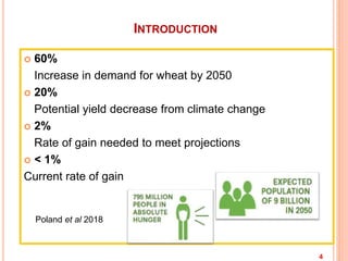
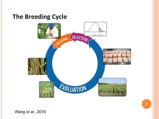
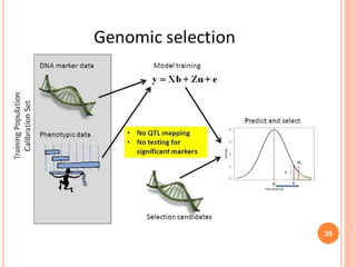
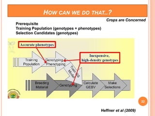
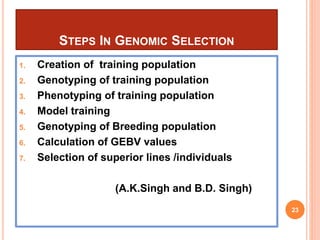
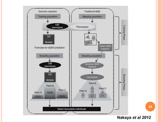
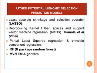
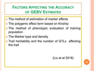
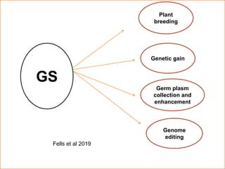
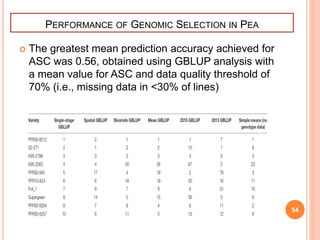
WELCOME
GENOMIC SELECTION FOR
CROP IMPROVEMENT
Presented by
G.Nagamani
RAD-18-38
Ph.D I year
Molecular biology and biotechnology
2
CONTENTS
 Introduction
 Evolution of genomic selection
 Procedure for genomic selection
 Advantages and limitations of GS
 Applications of GS in crop improvement
 Conclusion
 Future Prospects
3
INTRODUCTION
 60%
Increase in demand for wheat by 2050
 20%
Potential yield decrease from climate change
 2%
Rate of gain needed to meet projections
 < 1%
Current rate of gain
4
Poland et al 2018
5
Wang et al., 2015
Genetic gain /GA
Selection was played important role
in Human-plant co evolution
ΔG= Accuracy of selection X intensity of selection X genetic standard deviation
Generation interval
Selection in GS is usually based on Genomic estimated of breeding
values
Selections can take place in laboratory
6
Phenotypic selection is challenging for three
reasons
 phenotypes targeted by breeders are slow to
measure
 They are expensive to measure
 Experimental error and environment effects often
make the phenotype an imperfect guide to the
potential of the underlying genotype and therefore
the phenotypic measurement needs to be replicated
(Nawell and Jannink, 2014)
7
TRADITIONAL SELECTION
 Traits with low heritability
 Traits that are expressed late in individual’s
life
 Traits that can not be measured easily (ex:
disease resistance & quality traits)
 Time consuming and the rate of breeding
is slow
8
LIMITATIONS OF MAS
 The genes with big QTL effects
 The major success is only achieved with
the qualitative traits
 The biparental mapping populations used
in most QTL studies do not readily
translate to breeding applications
(A.K Singh and B.D. Singh)
9
10
EVOLUTION OF GENOMIC
SELECTION
11
HOW HAVE WE USED MARKERS FOR COMPLEX
TRAITS IN THE ERA OF LOW MARKER DENSITY?
Marker-assisted recurrent
selection
1.Make cross to form
biparental population of
progenies
2. Phenotype and genotype
3. Select markers and
estimate marker effects within
biparental population
4. Select and recombine
5. Repeat
12
(Lorenz, A)
WHAT IS THE BEST USE OF MARKER INFORMATION IN THE
ERA OF HIGH MARKER DENSITY?
 Combine progenies from entire breeding
population to estimate marker effects
 Exploit population-wide LD
 Minimize phenotyping
 Estimate allelic effects in context of entire breeding
population
 Use all marker information to capture small
allelic effects
 (Lorenz, A)
13
 The term ‘GS’ was first introduced by Haley and
Visscher at the 6th World Congress on Genetics Applied
to Livestock Production at Armidale, Australia in 1998
 GS was first propounded by Meuwissen et al (2001) :
Seminal paper ‘Meuwissen et al (2001) Prediction of
total genetic value using genome-wide dense marker
maps. Genetics 157: 1819-29.”
14
GENOMIC SELECTION
 Specialized form of MAS, in which information
from genotype data on marker alleles covering
the entire genome forms the basis of selection
 EBV: An estimate of the additive genetic merit for
a particular trait that an individual will pass on to its
descendant's.
 GEBVs: Prediction of the genetic merit of an
individual based on its genome.
15
 Trace all segments of the genome with markers
-Capture all QTL = all genetic variance
 Predict genomic breeding values as sum of
effects over all segments
 Genomic selection exploits LD.
 Genomic selection avoids bias in estimation of
effects due to multiple testing, as all effects fitted
simultaneously.
16
17
18
19
20
PRE-REQUISITE FOR THE INTRODUCTION OF
GS
The need for adequate and affordable
genotyping platforms
Relatively simple breeding schemes in
which selection of additive genetic effects
will generate useful results
Statistical methods
21
HOW CAN WE DO THAT..?
Prerequisite
Training Population (genotypes + phenotypes)
Selection Candidates (genotypes)
Crops are Concerned
Heffner et al (2009)
22
STEPS IN GENOMIC SELECTION
1. Creation of training population
2. Genotyping of training population
3. Phenotyping of training population
4. Model training
5. Genotyping of Breeding population
6. Calculation of GEBV values
7. Selection of superior lines /individuals
(A.K.Singh and B.D. Singh)
23
24
Nakaya et al 2012
25
TRAINING POPULATION
 Training of the GS model and for obtaining
estimates of the marker-associated effects
needed for estimation of GEBVs of
individuals/lines in the breeding population
 Low colineraity between markers
 Represnting the genetic diversity in
breeding population
26
CHARACTERISTICS OF TRAINING POPULATION
 Genetic composition
 Large population and parents or very recent
ancestors of breeding population
 Historical data or real population consisting of existing
individuals (Biparental crosses, double haploids, test
crosses and inbred lines)
 New training population for each breeding population
is ideal
27
POPULATION SIZE
 The accuracy of GEBV prediction
 low heritability trait
 Cross pollinated crops
 The ratio of training to breeding
population
High
28
MARKER DENSITY
 Large number of markers
 Maximum QTL affecting trait is in stronger LD
 Cross pollinated crops
 Low heritable traits
 GEBV accuracy improves with marker density
up to a point, beyond which there is little
improvement
 Evenly spaced, low-density markers may
predict GEBVs with lower accuracy
More
density
29
MARKER TYPE
 SNP (single nucleotide polymorphism)
 DArT (Diversity arrays technology)
 GBS (Genotyping by sequencing)
(Shamsad and Sharma , 2017) 30
SNP CHIP IN GENOMIC SELECTION
 variations detected at the level of a single
nucleotide base in the genome
 Abundant in nature. 1kb-2SNP.
 Availability of a wide array of genotyping platforms
with various multiplex capabilities
 Predicting differences in BVs
 NGS enabled millions of sequences reads to be
generated from a single run at a more affordable
cost
(Shamsad and Sharma , 2017) 31
32
GBS
 GBS accesses regulatory regions and sequence tag
mapping.
 Flexibility and low cost.
 GBS markers led to higher genomic prediction
accuracies.
 Impute missing data.
 Highly multiplexed
 Even for a species with a genome as challenging
as wheat (Absence of a reference genome)
(Shamsad and Sharma , 2017)
Elshire et al (2010)
33
GENOMIC SELECTION PREDICTION MODELS
1. Stepwise regression
2. Ridge regression
3. Bayesian estimation models
Meuwissen et al (2001) Prediction of total genetic value using
genome-wide densen marker maps. Genetics 157: 1819-29.
34
STEPWISE REGRESSION (SR)
 Select most significant markers on the basis of
arbitrary significant thresholds and non significant
markers effect equals to zero. (Lande and
Thompson, 1990)
 Estimate the effect of significant markers using
multiple regression Since, only a portion of the
genetic variance will be captured.
 Limitations :
 Detects only large effects and that cause
overestimation of significant effects (Goddard and
Hayes, 2007; Beavis, 1998 )
 SR resulted in low GEBVs accuracy due to limited
detection of QTLs.
(Meuwissen et al 2001)
35
RIDGE REGRESSION BLUP (RR-BLUP)
 Simultaneously select all marker effects rather than
categorizing into significant or having no effect
 Ridge regression shrinks all marker effects towards zero.
 The method makes the assumption that markers are
random effects with a equal variance. (Meuwissen et al
2001)
 Limitations :
 RR-BLUP incorrectly treats all effects equally which is
unrealistic. (Xu et al 2003)
 RR-BLUP Superior to SR 36
BAYESIAN REGRESSION (BR)
 Marker variance treated more realistically by
assuming specified prior distribution.
 BayesA: uses an inverted chi-square to
regress the marker variance towards zero.
 All marker effects are > 0 (Bayes A)
 BayesB:.
 Some marker effects can be = 0 (Bayes B)
 GEBV does not decline with an increase in marker
density
(Meuwissen et al 2001) 37
OTHER POTENTIAL GENOMIC SELECTION
PREDICTION MODELS
 Least absolute shrinkage and selection operator
(LASSO)
 Reproducing Kernel Hilbert spaces and support
vector machine regression. (RKHS) Gianola et al
(2006)
 Partial Least Squares regression & principle
component regression.
 RF (R package random forest)
 MVN EM Algorithm
38
39
FACTORS AFFECTING THE ACCURACY
OF GEBV ESTIMATES
 The method of estimation of marker effects
 The polygenic effect term based on Kinship
 The method of phenotypic evaluation of training
population
 The Marker type and density
 Trait heritability and the number of QTLs affecting
the trait
(Liu et al 2018)
40
ADVANTAGES
 Marker effects are estimated in training population
and QTL discovery and mapping is not required
 Greater gains per unit time than phenotypic
selection
 Increases the effectiveness of selection, particularly
for low heritability traits
 Reduce rate of inbreeding depression and loss of
genetic variability
 Shortens the length of breeding cycle
 Selection of hybrids for hybridization programme
 Allow GEBV estimation even for traits for which they
have never been tested
41
LIMITATIONS
 Still not become popular due to lack of evidences for
its practical use
 The potential value of GS should be assessed with
caution
 The marker effects and, as a result, GEBV estimates
may change due to changes in gene frequencies and
epistatic interactions
 Simulation models ignore epistatic effect
 knowledge about the genetic architecture of
quantitative traits is severely limited
 The selection response declines at a faster rate under
GS than with pedigree selection
 off-season/greenhouse facilities are required
 The need for genotyping of a large number of marker
42
GS VS MAS
Feature Genomic selection MAS
Targeted QTLs All QTLs affecting the trait QTLs with significant and large
effects
Basis of selection GEBVs estimated from marker
genotypes
Marker genotype
Number of markers
used
Large number of genome-wide
markers
Few markers linked to the
targeted QTLs
QTL discovery,
confirmation, and
validation
Not required; QTL effects
associated with the markers are
estimated
Necessary for successful MAS
Model training Necessary; based on a suitable
training population
Not required
Phenotypic evaluation Confined to the training
population
During QTL discovery,
confirmation, and
validation
Overall objective of the
breeding program
Improvement in the targeted
quantitative traits
Introgression/accumulation of
the targeted QTLs
GS
Plant
breeding
Genetic gain
Germ plasm
collection and
enhancement
Genome
editing
44
Fells et al 2019
PLANT BREEDING
 Creation of new variation and recurrent population
improvement
 The selection of superior inbred lines for variety
development
 Either with increased agronomic traits
 Biotic stress resistance
 Abiotic stress resistance
45
Rutkoski et al. 2010
GS SCHEME IN CROPS
46
A. K singh and B.D. singh
INCREASING GAIN THROUGH RAPID GENERATION
ADVANCEMENT AND GENOMIC SELECTION
 2.5 times more genetic gain
 DHs technology can be costly, at times inefficient in terms
of natural or chemical-induced chromosome doubling and
the breeder cannot select for basic traits during line
development
 In speed breeding costs associated with installation and
running of suitable facilities currently constrain the
widespread application of the tool
 GS and speed breeding could potentially increase genetic
gain significantly, compared to both classical phenotypic
selection and standard GS-based breeding schemes
(Voss-Fels et al. 2018a)
47
CASE STUDY
48
Carpenter et al., 2018
 Evaluation of GS for breeding ascochyta blight disease
resistance in a pea breeding program
 compared the ability of several GS models to predict
phenotypes, and explored the effects SNP quality and number
 GBS was used to genotype the training population
 Plant material – 215 lines from PFR
 Phenotyping traits : Disease severity score of Ascochyta
blight (ASC)
 Two field trails : 2013, 2015. (natural occuring field epidemics)
 randomized complete block design with three blocks;
 each block contained 3 rows and 77 columns.
 One breeding line (“Ashton,” Seminis) was used as a control
and planted in every 11th plot.
 Each plot was sown with 50 seeds in a single row.
49
 Genotyping
 GBS libraries were constructed according to the method of
Elshire et al. (2011)
 DNA (200 ng) was digested ApeKI enzyme Adaptors were
ligated to the digested DNA with barcoded and common
adaptors with T4 DNA ligase
 Ligation products were then amplified by PCR
 10 ml per amplified library were pooled, and purified were
sequenced using the Illumina HiSeq 2000 platform
 Raw data was assessed using FastQC for sequence quality
and presence of adapter read through.
 UNEAK software : SNP identification (74,738SNP)
 The hapmap files were imported into TASSEL v3.0.165 for
filtering on SNP and taxa quality
 SNPs at three thresholds for genotyping : 50, 70, and 90%
of lines have SNP data (<50, 30, and 10% missing data,
respectively) using R software
 150 lines training population
 50 breeding population 50
51
Results (phenotypic data)
2015 greater variation (range
1.7–4.7, mean 3.0) than in 2013
(range 2.7–4.5, mean 3.5).
Correlation (Pearson) between
the mean ASC scores from the
two field trials was only
moderate (r = 0.46)
COMPARISON OF DIFFERENT GS MODELS
52
COMPARISON OF SNP QUALITY THRESHOLDS
53
PERFORMANCE OF GENOMIC SELECTION IN PEA
 The greatest mean prediction accuracy achieved for
ASC was 0.56, obtained using GBLUP analysis with
a mean value for ASC and data quality threshold of
70% (i.e., missing data in <30% of lines)
54
GERMPLASM COLLECTION AND ENHANCEMENT
 Enhancing adaptive capacity
 Introgress novel allelic diversity which is absent in modern
elite germplasm pools using genetic resources (Huang
and Han 2014)
 But there is a lot of potentially useful variation locked in
gene banks
 Exotic accessions must be phenotyped, which is
technically and financially challenging
 Using genome-wide markers and GS principles, breeding
values for the exotic accessions can be determined and
used to specifically reinstate diversity for target traits in a
given germplasm pool
(Longin and Reif 2014)
55
56
Plant genome
Case study
 Wheat germplasm and phenotypic evaluation
 1163 hexaploid spring wheat accessions
 5 field experiments at 2 locations (2012,14)
 Nursery : High disease incidence pressure
 SNP genotyping
 Illumina iSelect 9K wheat assay
 5619 high-quality SNPs
 Prediction of GEBV and Assessment of Accuracy
 Effect of Training Population Size and Composition
1163, 210,478,640 as TP
 Genomic Selection with Marker Panels of Different Densities
5619 SNPs at at 3 levels of density
 A total of 1849, 543, and 322 SNP markers were retained for
M1cM, M5cM, and M10cM, with an average of 1 SNP per 3.2,
9.4, and 14.8 cM, respectively. 57
58
59
Marker density and training population
COMBINING GENOMIC SELECTION WITH
GENOME EDITING
 Reversal of deleterious mutations
 Lack of their complete removal is that selection is
constrained by LD with favorable alleles and limited
population sizes
 Prediction accuracies of traits could significantly be
improved when information about deleterious
alleles was used to inform GS models
60
61
CASE STUDY
 Objectives
 (i) the predicted responses to selection if one or two targeted
recombinations were to occur on each maize chromosome
 (ii) the extent to which the predicted responses with targeted
recombination vary among maize traits and populations
 (iii) the consistency of the ideal recombination points among maize
traits and populations
62
Materials and methods
Experiment 1
•180 recombinant inbreds (B73 × Mo17)
•Grain yield , moisture , plant height (cm), stalk lodging (%), root lodging(%),
and stover quality traits
•The field trials were conducted at four Minnesota locations in 2007.
•892 SNP loci
•160,560 data points for 180 recombinant inbreds and 892 SNP loci,
•546 (0.34%) were heterozygous
679 (0.42%) had missing data after projection : genomewide marker effects
-ridge regression-best linear unbiased prediction (RR-BLUP)
 Experiment 2
 10 Recombinant inbreds from 271 inbreds
 The 271 inbreds : anthesis date, plant height (cm), kernel
starch concentration (g kg-1), and kernel protein concentration
(g kg-1) at five Minnesota locations in 2011 and one Minnesota
location in 2012.
 Genomewide marker effects at 28,826 SNP loci were
previously calculated by Schaefer and Bernardo (2013) using
rrBLUP software in R
 Procedure
 (i) a multiplex CRISPR system induces mitotic double-strand
breaks at multiple target DNA sequences,
 (ii) cells with the desired loss-of-heterozygosity events are
screened (iii) the desired cells are regenerated into whole
plants that carry the targeted recombinations.
 From the regenerated plants, doubled haploids can be
developed 63
64
RESULTS
65
CONCLUSION
 the RETargeted values for maize yield and other
agronomic traits suggested that an ability to induce
one or two targeted recombinations per
chromosome may double the current selection
gains.
 Developing targeted recombination technology
therefore might be worthwhile, particularly given the
concerns that the current rates of increase in crop
productivity are not enough to meet the goal of
doubling global crop production by 2050
66
 Genotype × environment interactions
 Non-additive genetic variance
 In the presence of GEI and non additive genetic
variance, the substitution effects of QTL alleles will
change the crop breeding programmes.
 There will be changes in ranks of allele effects
associated with the changes in substitution effects are
associated with changes in ranking values of alleles
67
CHALLENGES TO THE SUCCESS OF GENOMIC
SELECTION IN CROPS
CURRENT STATUS
Sno Species NGS platform Trait Reference
1 Rice GBS
Grain yield ,
Floweringtime Spindel et al 2015
2 Wheat GBS
Stem rust
resistance, Plant
height Rutkoski et al 2014
3 Canola DArTSeq Floweing time Raman et al 2015
4 Wheat GBS
Grain yield,
protein content Isidro et al 2105
5 Grape vine GBS
yield and yield
related traits Fodor et al 2014
6 Rye grass GBS
plant herbage and
dry weight Favelle et al 2016
7 Wheat GBS
Fusarium head
Blight resistance Aruda et al 2016
68
CONCLUSION
 In this regard, GS has been suggested to have a potential
to fix all the genetic variation of complex traits
 Many studies have shown tremendous opportunities of
GS to increase genetic gain in plant breeding
 Revolution of inexpensive NGS technologies has resulted
in increasing number of crop genomes as well as
provides the low cost and high density SNP genotyping
69
FUTURE PROSPECTS
 The genomic sequencing cost further decreases and
WGS become feasible and cost effective for GS, there will
be further increase in the prediction accuracy of GS
 Develop appropriate statistical tools and software
 Data base for storing data generated through GS
 Guidelines for construction of training population.
70
Genomic selection for crop improvement

Genomic selection for crop improvement

  • 1.
  • 2.
    GENOMIC SELECTION FOR CROPIMPROVEMENT Presented by G.Nagamani RAD-18-38 Ph.D I year Molecular biology and biotechnology 2
  • 3.
    CONTENTS  Introduction  Evolutionof genomic selection  Procedure for genomic selection  Advantages and limitations of GS  Applications of GS in crop improvement  Conclusion  Future Prospects 3
  • 4.
    INTRODUCTION  60% Increase indemand for wheat by 2050  20% Potential yield decrease from climate change  2% Rate of gain needed to meet projections  < 1% Current rate of gain 4 Poland et al 2018
  • 5.
  • 6.
    Genetic gain /GA Selectionwas played important role in Human-plant co evolution ΔG= Accuracy of selection X intensity of selection X genetic standard deviation Generation interval Selection in GS is usually based on Genomic estimated of breeding values Selections can take place in laboratory 6
  • 7.
    Phenotypic selection ischallenging for three reasons  phenotypes targeted by breeders are slow to measure  They are expensive to measure  Experimental error and environment effects often make the phenotype an imperfect guide to the potential of the underlying genotype and therefore the phenotypic measurement needs to be replicated (Nawell and Jannink, 2014) 7
  • 8.
    TRADITIONAL SELECTION  Traitswith low heritability  Traits that are expressed late in individual’s life  Traits that can not be measured easily (ex: disease resistance & quality traits)  Time consuming and the rate of breeding is slow 8
  • 9.
    LIMITATIONS OF MAS The genes with big QTL effects  The major success is only achieved with the qualitative traits  The biparental mapping populations used in most QTL studies do not readily translate to breeding applications (A.K Singh and B.D. Singh) 9
  • 10.
  • 11.
  • 12.
    HOW HAVE WEUSED MARKERS FOR COMPLEX TRAITS IN THE ERA OF LOW MARKER DENSITY? Marker-assisted recurrent selection 1.Make cross to form biparental population of progenies 2. Phenotype and genotype 3. Select markers and estimate marker effects within biparental population 4. Select and recombine 5. Repeat 12 (Lorenz, A)
  • 13.
    WHAT IS THEBEST USE OF MARKER INFORMATION IN THE ERA OF HIGH MARKER DENSITY?  Combine progenies from entire breeding population to estimate marker effects  Exploit population-wide LD  Minimize phenotyping  Estimate allelic effects in context of entire breeding population  Use all marker information to capture small allelic effects  (Lorenz, A) 13
  • 14.
     The term‘GS’ was first introduced by Haley and Visscher at the 6th World Congress on Genetics Applied to Livestock Production at Armidale, Australia in 1998  GS was first propounded by Meuwissen et al (2001) : Seminal paper ‘Meuwissen et al (2001) Prediction of total genetic value using genome-wide dense marker maps. Genetics 157: 1819-29.” 14
  • 15.
    GENOMIC SELECTION  Specializedform of MAS, in which information from genotype data on marker alleles covering the entire genome forms the basis of selection  EBV: An estimate of the additive genetic merit for a particular trait that an individual will pass on to its descendant's.  GEBVs: Prediction of the genetic merit of an individual based on its genome. 15
  • 16.
     Trace allsegments of the genome with markers -Capture all QTL = all genetic variance  Predict genomic breeding values as sum of effects over all segments  Genomic selection exploits LD.  Genomic selection avoids bias in estimation of effects due to multiple testing, as all effects fitted simultaneously. 16
  • 17.
  • 18.
  • 19.
  • 20.
  • 21.
    PRE-REQUISITE FOR THEINTRODUCTION OF GS The need for adequate and affordable genotyping platforms Relatively simple breeding schemes in which selection of additive genetic effects will generate useful results Statistical methods 21
  • 22.
    HOW CAN WEDO THAT..? Prerequisite Training Population (genotypes + phenotypes) Selection Candidates (genotypes) Crops are Concerned Heffner et al (2009) 22
  • 23.
    STEPS IN GENOMICSELECTION 1. Creation of training population 2. Genotyping of training population 3. Phenotyping of training population 4. Model training 5. Genotyping of Breeding population 6. Calculation of GEBV values 7. Selection of superior lines /individuals (A.K.Singh and B.D. Singh) 23
  • 24.
  • 25.
    Nakaya et al2012 25
  • 26.
    TRAINING POPULATION  Trainingof the GS model and for obtaining estimates of the marker-associated effects needed for estimation of GEBVs of individuals/lines in the breeding population  Low colineraity between markers  Represnting the genetic diversity in breeding population 26
  • 27.
    CHARACTERISTICS OF TRAININGPOPULATION  Genetic composition  Large population and parents or very recent ancestors of breeding population  Historical data or real population consisting of existing individuals (Biparental crosses, double haploids, test crosses and inbred lines)  New training population for each breeding population is ideal 27
  • 28.
    POPULATION SIZE  Theaccuracy of GEBV prediction  low heritability trait  Cross pollinated crops  The ratio of training to breeding population High 28
  • 29.
    MARKER DENSITY  Largenumber of markers  Maximum QTL affecting trait is in stronger LD  Cross pollinated crops  Low heritable traits  GEBV accuracy improves with marker density up to a point, beyond which there is little improvement  Evenly spaced, low-density markers may predict GEBVs with lower accuracy More density 29
  • 30.
    MARKER TYPE  SNP(single nucleotide polymorphism)  DArT (Diversity arrays technology)  GBS (Genotyping by sequencing) (Shamsad and Sharma , 2017) 30
  • 31.
    SNP CHIP INGENOMIC SELECTION  variations detected at the level of a single nucleotide base in the genome  Abundant in nature. 1kb-2SNP.  Availability of a wide array of genotyping platforms with various multiplex capabilities  Predicting differences in BVs  NGS enabled millions of sequences reads to be generated from a single run at a more affordable cost (Shamsad and Sharma , 2017) 31
  • 32.
  • 33.
    GBS  GBS accessesregulatory regions and sequence tag mapping.  Flexibility and low cost.  GBS markers led to higher genomic prediction accuracies.  Impute missing data.  Highly multiplexed  Even for a species with a genome as challenging as wheat (Absence of a reference genome) (Shamsad and Sharma , 2017) Elshire et al (2010) 33
  • 34.
    GENOMIC SELECTION PREDICTIONMODELS 1. Stepwise regression 2. Ridge regression 3. Bayesian estimation models Meuwissen et al (2001) Prediction of total genetic value using genome-wide densen marker maps. Genetics 157: 1819-29. 34
  • 35.
    STEPWISE REGRESSION (SR) Select most significant markers on the basis of arbitrary significant thresholds and non significant markers effect equals to zero. (Lande and Thompson, 1990)  Estimate the effect of significant markers using multiple regression Since, only a portion of the genetic variance will be captured.  Limitations :  Detects only large effects and that cause overestimation of significant effects (Goddard and Hayes, 2007; Beavis, 1998 )  SR resulted in low GEBVs accuracy due to limited detection of QTLs. (Meuwissen et al 2001) 35
  • 36.
    RIDGE REGRESSION BLUP(RR-BLUP)  Simultaneously select all marker effects rather than categorizing into significant or having no effect  Ridge regression shrinks all marker effects towards zero.  The method makes the assumption that markers are random effects with a equal variance. (Meuwissen et al 2001)  Limitations :  RR-BLUP incorrectly treats all effects equally which is unrealistic. (Xu et al 2003)  RR-BLUP Superior to SR 36
  • 37.
    BAYESIAN REGRESSION (BR) Marker variance treated more realistically by assuming specified prior distribution.  BayesA: uses an inverted chi-square to regress the marker variance towards zero.  All marker effects are > 0 (Bayes A)  BayesB:.  Some marker effects can be = 0 (Bayes B)  GEBV does not decline with an increase in marker density (Meuwissen et al 2001) 37
  • 38.
    OTHER POTENTIAL GENOMICSELECTION PREDICTION MODELS  Least absolute shrinkage and selection operator (LASSO)  Reproducing Kernel Hilbert spaces and support vector machine regression. (RKHS) Gianola et al (2006)  Partial Least Squares regression & principle component regression.  RF (R package random forest)  MVN EM Algorithm 38
  • 39.
  • 40.
    FACTORS AFFECTING THEACCURACY OF GEBV ESTIMATES  The method of estimation of marker effects  The polygenic effect term based on Kinship  The method of phenotypic evaluation of training population  The Marker type and density  Trait heritability and the number of QTLs affecting the trait (Liu et al 2018) 40
  • 41.
    ADVANTAGES  Marker effectsare estimated in training population and QTL discovery and mapping is not required  Greater gains per unit time than phenotypic selection  Increases the effectiveness of selection, particularly for low heritability traits  Reduce rate of inbreeding depression and loss of genetic variability  Shortens the length of breeding cycle  Selection of hybrids for hybridization programme  Allow GEBV estimation even for traits for which they have never been tested 41
  • 42.
    LIMITATIONS  Still notbecome popular due to lack of evidences for its practical use  The potential value of GS should be assessed with caution  The marker effects and, as a result, GEBV estimates may change due to changes in gene frequencies and epistatic interactions  Simulation models ignore epistatic effect  knowledge about the genetic architecture of quantitative traits is severely limited  The selection response declines at a faster rate under GS than with pedigree selection  off-season/greenhouse facilities are required  The need for genotyping of a large number of marker 42
  • 43.
    GS VS MAS FeatureGenomic selection MAS Targeted QTLs All QTLs affecting the trait QTLs with significant and large effects Basis of selection GEBVs estimated from marker genotypes Marker genotype Number of markers used Large number of genome-wide markers Few markers linked to the targeted QTLs QTL discovery, confirmation, and validation Not required; QTL effects associated with the markers are estimated Necessary for successful MAS Model training Necessary; based on a suitable training population Not required Phenotypic evaluation Confined to the training population During QTL discovery, confirmation, and validation Overall objective of the breeding program Improvement in the targeted quantitative traits Introgression/accumulation of the targeted QTLs
  • 44.
    GS Plant breeding Genetic gain Germ plasm collectionand enhancement Genome editing 44 Fells et al 2019
  • 45.
    PLANT BREEDING  Creationof new variation and recurrent population improvement  The selection of superior inbred lines for variety development  Either with increased agronomic traits  Biotic stress resistance  Abiotic stress resistance 45 Rutkoski et al. 2010
  • 46.
    GS SCHEME INCROPS 46 A. K singh and B.D. singh
  • 47.
    INCREASING GAIN THROUGHRAPID GENERATION ADVANCEMENT AND GENOMIC SELECTION  2.5 times more genetic gain  DHs technology can be costly, at times inefficient in terms of natural or chemical-induced chromosome doubling and the breeder cannot select for basic traits during line development  In speed breeding costs associated with installation and running of suitable facilities currently constrain the widespread application of the tool  GS and speed breeding could potentially increase genetic gain significantly, compared to both classical phenotypic selection and standard GS-based breeding schemes (Voss-Fels et al. 2018a) 47
  • 48.
  • 49.
     Evaluation ofGS for breeding ascochyta blight disease resistance in a pea breeding program  compared the ability of several GS models to predict phenotypes, and explored the effects SNP quality and number  GBS was used to genotype the training population  Plant material – 215 lines from PFR  Phenotyping traits : Disease severity score of Ascochyta blight (ASC)  Two field trails : 2013, 2015. (natural occuring field epidemics)  randomized complete block design with three blocks;  each block contained 3 rows and 77 columns.  One breeding line (“Ashton,” Seminis) was used as a control and planted in every 11th plot.  Each plot was sown with 50 seeds in a single row. 49
  • 50.
     Genotyping  GBSlibraries were constructed according to the method of Elshire et al. (2011)  DNA (200 ng) was digested ApeKI enzyme Adaptors were ligated to the digested DNA with barcoded and common adaptors with T4 DNA ligase  Ligation products were then amplified by PCR  10 ml per amplified library were pooled, and purified were sequenced using the Illumina HiSeq 2000 platform  Raw data was assessed using FastQC for sequence quality and presence of adapter read through.  UNEAK software : SNP identification (74,738SNP)  The hapmap files were imported into TASSEL v3.0.165 for filtering on SNP and taxa quality  SNPs at three thresholds for genotyping : 50, 70, and 90% of lines have SNP data (<50, 30, and 10% missing data, respectively) using R software  150 lines training population  50 breeding population 50
  • 51.
    51 Results (phenotypic data) 2015greater variation (range 1.7–4.7, mean 3.0) than in 2013 (range 2.7–4.5, mean 3.5). Correlation (Pearson) between the mean ASC scores from the two field trials was only moderate (r = 0.46)
  • 52.
  • 53.
    COMPARISON OF SNPQUALITY THRESHOLDS 53
  • 54.
    PERFORMANCE OF GENOMICSELECTION IN PEA  The greatest mean prediction accuracy achieved for ASC was 0.56, obtained using GBLUP analysis with a mean value for ASC and data quality threshold of 70% (i.e., missing data in <30% of lines) 54
  • 55.
    GERMPLASM COLLECTION ANDENHANCEMENT  Enhancing adaptive capacity  Introgress novel allelic diversity which is absent in modern elite germplasm pools using genetic resources (Huang and Han 2014)  But there is a lot of potentially useful variation locked in gene banks  Exotic accessions must be phenotyped, which is technically and financially challenging  Using genome-wide markers and GS principles, breeding values for the exotic accessions can be determined and used to specifically reinstate diversity for target traits in a given germplasm pool (Longin and Reif 2014) 55
  • 56.
  • 57.
     Wheat germplasmand phenotypic evaluation  1163 hexaploid spring wheat accessions  5 field experiments at 2 locations (2012,14)  Nursery : High disease incidence pressure  SNP genotyping  Illumina iSelect 9K wheat assay  5619 high-quality SNPs  Prediction of GEBV and Assessment of Accuracy  Effect of Training Population Size and Composition 1163, 210,478,640 as TP  Genomic Selection with Marker Panels of Different Densities 5619 SNPs at at 3 levels of density  A total of 1849, 543, and 322 SNP markers were retained for M1cM, M5cM, and M10cM, with an average of 1 SNP per 3.2, 9.4, and 14.8 cM, respectively. 57
  • 58.
  • 59.
    59 Marker density andtraining population
  • 60.
    COMBINING GENOMIC SELECTIONWITH GENOME EDITING  Reversal of deleterious mutations  Lack of their complete removal is that selection is constrained by LD with favorable alleles and limited population sizes  Prediction accuracies of traits could significantly be improved when information about deleterious alleles was used to inform GS models 60
  • 61.
  • 62.
     Objectives  (i)the predicted responses to selection if one or two targeted recombinations were to occur on each maize chromosome  (ii) the extent to which the predicted responses with targeted recombination vary among maize traits and populations  (iii) the consistency of the ideal recombination points among maize traits and populations 62 Materials and methods Experiment 1 •180 recombinant inbreds (B73 × Mo17) •Grain yield , moisture , plant height (cm), stalk lodging (%), root lodging(%), and stover quality traits •The field trials were conducted at four Minnesota locations in 2007. •892 SNP loci •160,560 data points for 180 recombinant inbreds and 892 SNP loci, •546 (0.34%) were heterozygous 679 (0.42%) had missing data after projection : genomewide marker effects -ridge regression-best linear unbiased prediction (RR-BLUP)
  • 63.
     Experiment 2 10 Recombinant inbreds from 271 inbreds  The 271 inbreds : anthesis date, plant height (cm), kernel starch concentration (g kg-1), and kernel protein concentration (g kg-1) at five Minnesota locations in 2011 and one Minnesota location in 2012.  Genomewide marker effects at 28,826 SNP loci were previously calculated by Schaefer and Bernardo (2013) using rrBLUP software in R  Procedure  (i) a multiplex CRISPR system induces mitotic double-strand breaks at multiple target DNA sequences,  (ii) cells with the desired loss-of-heterozygosity events are screened (iii) the desired cells are regenerated into whole plants that carry the targeted recombinations.  From the regenerated plants, doubled haploids can be developed 63
  • 64.
  • 65.
  • 66.
    CONCLUSION  the RETargetedvalues for maize yield and other agronomic traits suggested that an ability to induce one or two targeted recombinations per chromosome may double the current selection gains.  Developing targeted recombination technology therefore might be worthwhile, particularly given the concerns that the current rates of increase in crop productivity are not enough to meet the goal of doubling global crop production by 2050 66
  • 67.
     Genotype ×environment interactions  Non-additive genetic variance  In the presence of GEI and non additive genetic variance, the substitution effects of QTL alleles will change the crop breeding programmes.  There will be changes in ranks of allele effects associated with the changes in substitution effects are associated with changes in ranking values of alleles 67 CHALLENGES TO THE SUCCESS OF GENOMIC SELECTION IN CROPS
  • 68.
    CURRENT STATUS Sno SpeciesNGS platform Trait Reference 1 Rice GBS Grain yield , Floweringtime Spindel et al 2015 2 Wheat GBS Stem rust resistance, Plant height Rutkoski et al 2014 3 Canola DArTSeq Floweing time Raman et al 2015 4 Wheat GBS Grain yield, protein content Isidro et al 2105 5 Grape vine GBS yield and yield related traits Fodor et al 2014 6 Rye grass GBS plant herbage and dry weight Favelle et al 2016 7 Wheat GBS Fusarium head Blight resistance Aruda et al 2016 68
  • 69.
    CONCLUSION  In thisregard, GS has been suggested to have a potential to fix all the genetic variation of complex traits  Many studies have shown tremendous opportunities of GS to increase genetic gain in plant breeding  Revolution of inexpensive NGS technologies has resulted in increasing number of crop genomes as well as provides the low cost and high density SNP genotyping 69
  • 70.
    FUTURE PROSPECTS  Thegenomic sequencing cost further decreases and WGS become feasible and cost effective for GS, there will be further increase in the prediction accuracy of GS  Develop appropriate statistical tools and software  Data base for storing data generated through GS  Guidelines for construction of training population. 70