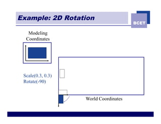
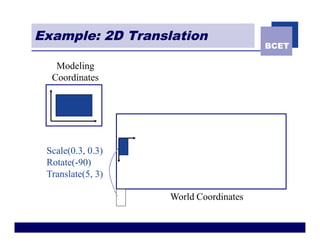
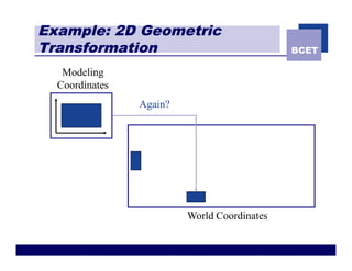
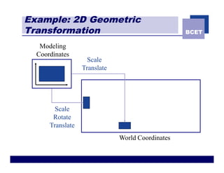
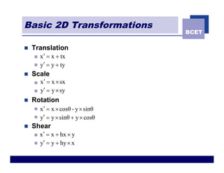
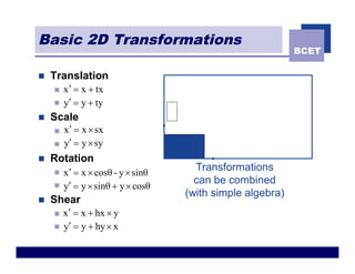
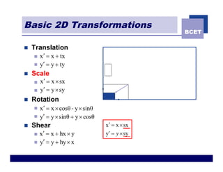
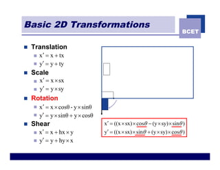
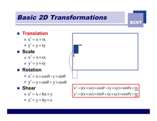
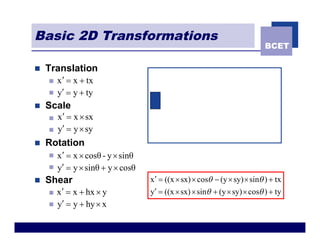
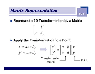
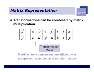
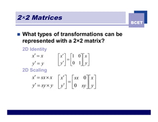
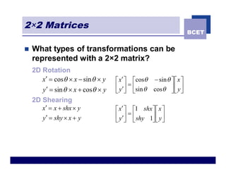
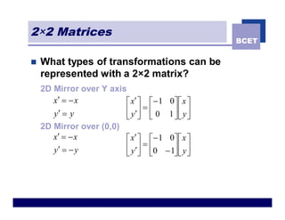
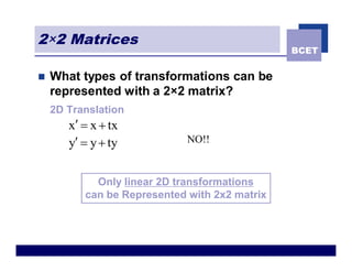
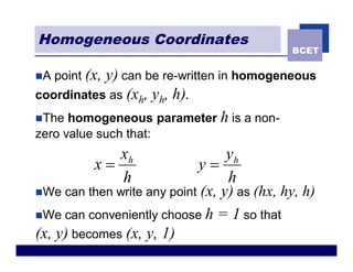
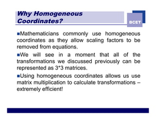
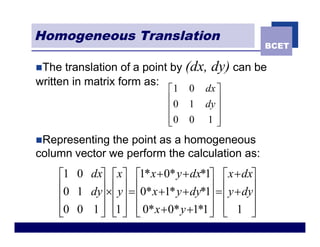
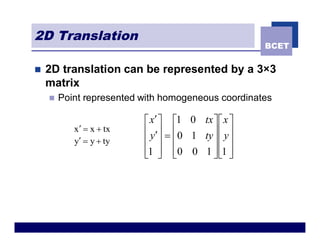
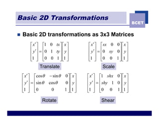
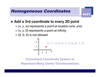
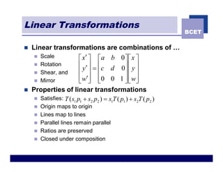
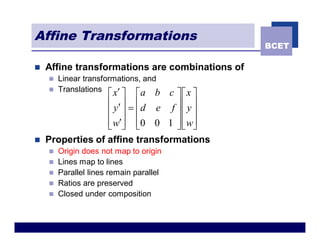
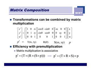
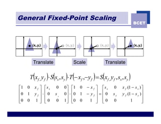
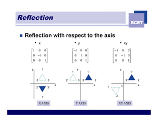
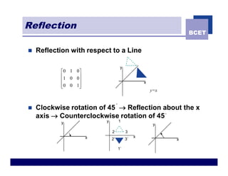
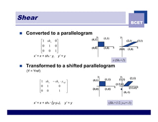
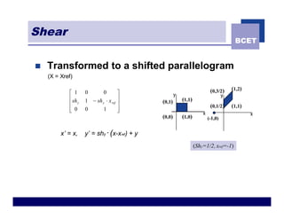
Graphics


 2D Geometric
Transformations

  Sudipta Mondal


                      sudipta.hit@gmail.com
Contents
                                                   BCET

n   Definition & Motivation
n   2D Geometric Transformation
    n Translation
    n Rotation
    n Scaling
n   Matrix Representation
n   Homogeneous Coordinates
n   Matrix Composition
n   Composite Transformations
    n Pivot-Point Rotation
    n General Fixed-Point Scaling
    n Reflection and Shearing
    n Transformations Between Coordinate Systems
Geometric Transformation
                                            BCET


n   Definition
    n   Translation, Rotation, Scaling.


n   Motivation – Why do we need geometric
    transformations in CG?
    n   As a viewing aid
    n   As a modeling tool
    n   As an image manipulation tool
Example: 2D Geometric
Transformation                       BCET

   Modeling
  Coordinates


                 World Coordinates
Example: 2D Scaling
                                       BCET

   Modeling
  Coordinates


 Scale(0.3, 0.3)


                   World Coordinates
Example: 2D Rotation
                                       BCET

   Modeling
  Coordinates


 Scale(0.3, 0.3)
 Rotate(-90)


                   World Coordinates
Example: 2D Translation
                                       BCET

   Modeling
  Coordinates


 Scale(0.3, 0.3)
 Rotate(-90)
 Translate(5, 3)

                   World Coordinates
Example: 2D Geometric
Transformation                               BCET

   Modeling
  Coordinates
                Again?


                         World Coordinates
Example: 2D Geometric
Transformation                                    BCET

   Modeling
  Coordinates
                    Scale
                  Translate


        Scale
       Rotate
      Translate
                              World Coordinates
Basic 2D Transformations
                                    BCET

n   Translation
    n   x ¢ = x + tx
    n   y¢ = y + ty
n   Scale
    n   x¢ = x ´ sx
    n   y¢ = y ´ sy
n   Rotation
    n   x ¢ = x ´ cosθ - y ´ sinθ
    n   y¢ = y ´ sinθ + y ´ cosθ
n   Shear
    n   x ¢ = x + hx ´ y
    n   y¢ = y + hy ´ x
Basic 2D Transformations
                                                            BCET

n   Translation
    n   x ¢ = x + tx
    n   y¢ = y + ty
n   Scale
    n   x¢ = x ´ sx
    n   y¢ = y ´ sy
n   Rotation
    n   x ¢ = x ´ cosθ - y ´ sinθ
                                      Transformations
                                      can be combined
    n   y¢ = y ´ sinθ + y ´ cosθ
                                    (with simple algebra)
n   Shear
    n   x ¢ = x + hx ´ y
    n   y¢ = y + hy ´ x
Basic 2D Transformations
                                                   BCET

n   Translation
    n   x ¢ = x + tx
    n   y¢ = y + ty
n   Scale
    n   x¢ = x ´ sx
    n   y¢ = y ´ sy
n   Rotation
    n   x ¢ = x ´ cosθ - y ´ sinθ
    n   y¢ = y ´ sinθ + y ´ cosθ
n   Shear                           x ¢ = x ´ sx
    n   x ¢ = x + hx ´ y            y¢ = y ´ sy
    n   y¢ = y + hy ´ x
Basic 2D Transformations
                                                                            BCET

n   Translation
    n   x ¢ = x + tx
    n   y¢ = y + ty
n   Scale
    n   x¢ = x ´ sx
    n   y¢ = y ´ sy
n   Rotation
    n   x ¢ = x ´ cosθ - y ´ sinθ
    n   y¢ = y ´ sinθ + y ´ cosθ
n   Shear                           x ¢ = ((x ´ sx) ´ cosq - (y ´ sy) ´ sinq )
    n   x ¢ = x + hx ´ y            y¢ = ((x ´ sx) ´ sinq + (y ´ sy) ´ cosq )
    n   y¢ = y + hy ´ x
Basic 2D Transformations
                                                                             BCET

n   Translation
    n   x ¢ = x + tx
    n   y¢ = y + ty
n   Scale
    n   x¢ = x ´ sx
    n   y¢ = y ´ sy
n   Rotation
    n   x ¢ = x ´ cosθ - y ´ sinθ
    n   y¢ = y ´ sinθ + y ´ cosθ
n   Shear                           x ¢ = ((x ´ sx) ´ cosq - (y ´ sy) ´ sinq ) + tx
    n   x ¢ = x + hx ´ y            y¢ = ((x ´ sx) ´ sinq + (y ´ sy) ´ cosq ) + ty
    n   y¢ = y + hy ´ x
Matrix Representation
                                                    BCET


n   Represent a 2D Transformation by a Matrix
                 éa b ù
                 êc d ú
                 ë    û
n   Apply the Transformation to a Point
       x¢ = ax + by         é x¢ ù é a b ù é x ù
       y¢ = cx + dy         ê y ¢ú = êc d ú ê y ú
                            ë û ë         ûë û
                      Transformation
                                                     Point
                          Matrix
Matrix Representation
                                                    BCET


n   Transformations can be combined by matrix
    multiplication

       é x¢ ù é a b ù ée      f ù éi j ù é x ù
       ê y ¢ú = ê c d ú ê g     ú êk l ú ê y ú
                              hû ë
       ë û ë          ûë               ûë û
                      Transformation
                          Matrix
      Matrices are a convenient and efficient way
      to represent a sequence of transformations
2×2 Matrices
                                              BCET


n   What types of transformations can be
    represented with a 2×2 matrix?
    2D Identity
        x¢ = x        é x¢ ù é1 0ù é x ù
                      ê y¢ú = ê0 1ú ê y ú
        y¢ = y        ë û ë       ûë û
    2D Scaling
        x¢ = sx ´ x   é x¢ ù é sx 0 ù é x ù
        y¢ = sy ´ y   ê y¢ú = ê0 sy ú ê y ú
                      ë û ë         ûë û
2×2 Matrices
                                                                   BCET


n   What types of transformations can be
    represented with a 2×2 matrix?
    2D Rotation
       x¢ = cos q ´ x - sin q ´ y   é x¢ ù écosq - sin q ù é x ù
                                    ê y¢ú = êsin q cosq ú ê y ú
       y¢ = sin q ´ x + cosq ´ y    ë û ë                ûë û
    2D Shearing
       x¢ = x + shx ´ y             é x¢ ù é1 shx ù é x ù
       y¢ = shy ´ x + y             ê y¢ú = ê shy 1ú ê y ú
                                    ë û ë          ûë û
2×2 Matrices
                                                     BCET


n   What types of transformations can be
    represented with a 2×2 matrix?
    2D Mirror over Y axis
       x¢ = - x          é x¢ ù é - 1    0ù é x ù
       y¢ = y            ê y ¢ú = ê 0    1 úê yú
                         ë û ë             ûë û
    2D Mirror over (0,0)
       x¢ = - x          é x¢ ù é - 1    0ù é x ù
       y¢ = - y          ê y ¢ú = ê 0   - 1ú ê y ú
                         ë û ë             ûë û
2×2 Matrices
                                               BCET


n   What types of transformations can be
    represented with a 2×2 matrix?
    2D Translation
       x¢ = x + tx
       y¢ = y + ty           NO!!


            Only linear 2D transformations
          can be Represented with 2x2 matrix
Homogeneous Coordinates
                                             BCET

nA   point (x,
           y) can be re-written in homogeneous
coordinates as (xh, yh, h).
nThe homogeneous parameter h is a non-
zero value such that:
               xh                 yh
            x=              y=
               h                  h
nWe can then write any point (x, y) as (hx, hy, h)

nWe can conveniently choose h = 1 so that
(x, y) becomes (x, y, 1)
Why Homogeneous
Coordinates?                                   BCET


nMathematicians      commonly use homogeneous
coordinates as they allow scaling factors to be
removed from equations.
nWe will see in a moment that all of the
transformations we discussed previously can be
represented as 3*3 matrices.
nUsing homogeneous coordinates allows us use
matrix multiplication to calculate transformations –
extremely efficient!
Homogeneous Translation
                                                     BCET

nThe  translation of a point by (dx,   dy) can be
written in matrix form as:
                             é1   0   dx ù
                             ê0   1   dy ú
                             ê           ú
                             ê0
                             ë    0   1ú û
nRepresenting the point as a homogeneous
column vector we perform the calculation as:
    é1 0 dxù éxù é1* x + 0* y + dx*1ù éx + dxù
    ê0 1 dyú ´êyú = ê0* x +1* y + dy*1ú = êy + dyú
    ê      ú ê ú ê                    ú ê        ú
    ê0 0 1 ú ê1 ú ê 0* x + 0* y +1*1 ú ë 1 ú
    ë      û ë û ë                    û ê        û
2D Translation
                                                    BCET

n   2D translation can be represented by a 3×3
    matrix
    n   Point represented with homogeneous coordinates

                          é x¢ ù é1 0 tx ù é x ù
           x ¢ = x + tx   ê y¢ú = ê0 1 ty ú ê y ú
           y¢ = y + ty    ê ú ê           úê ú
                          ê1 ú ê0 0 1 ú ê1 ú
                          ë û ë           ûë û
Basic 2D Transformations
                                                                BCET


n   Basic 2D transformations as 3x3 Matrices
        é x¢ ù é1 0 tx ù é x ù       é x¢ ù ésx 0 0 ù é x ù
        ê y¢ú = ê0 1 ty ú ê y ú      ê y¢ú = ê0 sy 0ú ê y ú
        ê ú ê           úê ú         ê ú ê          úê ú
        ê1 ú ê0 0 1 ú ê1 ú
        ë û ë           ûë û         ê1 ú ê0 0 1 ú ê1 ú
                                     ë û ë          ûë û
             Translate                       Scale
    é x¢ ù écosq - sin q 0 ù é x ù   é x¢ ù é1 shx 0 ù é x ù
    ê y¢ú = êsin q cosq  0ú ê y ú    ê y¢ú = ê shy 1 0ú ê y ú
    ê ú ê                  úê ú      ê ú ê            úê ú
    ê1 ú ê0
    ë û ë           0    1 ú ë1 ú
                           ûê û      ê1 ú ê0 0 1ú ê1 ú
                                     ë û ë            ûë û

               Rotate                        Shear
Homogeneous Coordinates
                                                                       BCET


n   Add a 3rd coordinate to every 2D point
    n   (x, y, w) represents a point at location (x/w, y/w)
    n   (x, y, 0) represents a point at infinity
    n   (0, 0, 0) is not allowed
                          y
                      2
                                      (2, 1, 1) or (4, 2, 2) or (6, 3, 3)
                      1
                                         x
                              1   2

            Convenient Coordinate System to
          Represent Many Useful Transformations
Linear Transformations
                                                            BCET

n   Linear transformations are combinations of …
     n Scale
                         é x¢ ù é a b 0 ù é x ù
     n Rotation          ê y ¢ ú = êc d 0 ú ê y ú
     n Shear, and        ê ú ê              úê ú
     n Mirror            ê w¢ú ê0 0 1 ú ê wû
                         ë û ë              ûë ú
n   Properties of linear transformations
     n Satisfies: T ( s p + s p ) = s T ( p ) + s T ( p )
                       1 1      2 2   1    1     2     2
    n   Origin maps to origin
    n   Lines map to lines
    n   Parallel lines remain parallel
    n   Ratios are preserved
    n   Closed under composition
Affine Transformations
                                                 BCET

n   Affine transformations are combinations of
    n Linear transformations, and
    n Translations
                     x¢
                  é ù é      a bc ùéx ù
                  ê y¢ ú = êd e f ú ê y ú
                  ê ú ê           úê ú
                  ê w¢ú ê0 0 1 ú ê wú
                  ë û ë           ûë û
n   Properties of affine transformations
    n   Origin does not map to origin
    n   Lines map to lines
    n   Parallel lines remain parallel
    n   Ratios are preserved
    n   Closed under composition
Matrix Composition
                                                                 BCET


n   Transformations can be combined by matrix
    multiplication
         é x¢ ù æ é1 0 tx ù écos θ - sinθ 0 ù ésx 0 0ù ö é x ù
         ê y¢ ú = ç ê0 1 ty ú ê sinθ cosθ 0ú ê0 sy 0 ú ÷ ê y ú
         ê ú çê             úê              úê       ú ÷ê ú
         ê w¢ú ç ê0 0 1 ú ê 0
         ë û èë             ûë        0   1 ú ê0 0 1 ú ÷ ê w ú
                                            ûë       û øë û
         p¢ =     T(tx, ty)      R(q )      S(sx, sy)      p
n   Efficiency with premultiplication
    n   Matrix multiplication is associative
        p¢ = (T ´ (R ´ (S ´ p)))            p¢ = (T ´ R ´ S) ´ p
Matrix Composition
                                                     BCET


n   Rotate by q around arbitrary point (a,b)
    n   M = T(a, b) ´ R(θ ) ´ T(-a,-b)
                                             (a,b)


n   Scale by sx, sy around arbitrary point (a,b)
    n   M = T(a, b) ´ S(sx, sy) ´ T(-a,-b)

                                             (a,b)
Inverse Transformations
                                             BCET


nTransformations  can easily be reversed using
inverse transformations

      é1 0 - dxù
   -1 ê        ú              é1      ù
  T = ê0 1 - dyú              ês 0 0ú
      ê0 0 1 ú
      ë        û              êx      ú
                           -1 ê   1 ú
                          S = 0      0
      é cos sinq 0ù
          q                   ê   sy ú
   -1 ê           ú           ê 0 0 1ú
  R = ê-sinq cos 0ú
               q              ê       ú
      ê 0                     ë       û
      ë       0 1úû
Pivot-Point Rotation
                                                                    BCET


           (xr,yr)            (xr,yr)             (xr,yr)            (xr,yr)


           Translate               Rotate               Translate

           T (xr , yr ) × R(q ) ×T (- xr ,-yr ) = R(xr , yr ,q )
é1 0 xr ù écosq - sinq 0ù é1 0 - xr ù écosq - sinq xr (1 - cosq ) + yr sinq ù
ê0 1 y ú × êsinq cosq 0ú × ê0 1 - y ú = êsinq cosq y (1 - cosq ) - x sinq ú
ê     rú ê              ú ê        rú ê             r                r      ú
ê0 0 1 û ê 0
ë       ú ë        0   1ú ê0 0 1 ú ê 0
                        û ë         û ë        0              1             ú
                                                                            û
General Fixed-Point Scaling
                                                                                 BCET


          (xf,yf)                (xf,yf)                 (xf,yf)                 (xf,yf)


           Translate                   Scale                 Translate


         T (xf , y f )× S(sx , sy )×T (- x f ,-y f ) = S(x f , y f , sx , sy )
é1   0      xf ù és x     0     0 ù é1     0    - x f ù és x       0    x f (1 - s x ) ù
ê0   1      yf ú×ê0       sy    0 ú × ê0   1    - yf ú = ê0        sy   y f (1 - s y ) ú
ê              ú ê                ú ê                 ú ê                              ú
ê0
ë    0       1 ú ê0
               û ë         0    1 ú ê0
                                  û ë      0      1 ú ê0
                                                      û ë          0          1        ú
                                                                                       û
Reflection
                                                                                     BCET


n   Reflection with respect to the axis
          •       x                         •   y                          •    xy

      é1 0 0ù                           é- 1 0 0ù                     é - 1 0 0ù
      ê0 - 1 0 ú                        ê 0 1 0ú                      ê 0 - 1 0ú
      ê        ú                        ê       ú                     ê        ú
      ê0 0 1 ú
      ë        û                        ê 0 0 1ú
                                        ë       û                     ê0
                                                                      ë     0 1ú
                                                                               û

      y               1                         y                          y
                                        1                1’                          1’


              2            3        2           3   3’        2                 3’        2
                                x                             x             3             x
          2’               3’                                     1


                      1’                                               2

                  X AXIS                    Y AXIS                         XY AXIS
Reflection
                                                                   BCET


n   Reflection with respect to a Line

                                        y
           é0 1 0 ù
           ê1 0 0 ú
           ê      ú                                  x
           ê0 0 1 ú
           ë      û
                                                         y=x


                                   °
n   Clockwise rotation of 45 ® Reflection about the x
    axis ® Counterclockwise rotation of 45 °
           y              y            1
                                                          y
                              2             3
                      x                          x
                              2’            3’                 x

                                       1’
Shear
                                                                                    BCET

n   Converted to a parallelogram
                                                  y    (1,1)           y
                                              (0,1)
               é1 sh x 0ù                                                      (2,1)        (3,1)
               ê0 1 0 ú
               ê           ú                  (0,0)    (1,0)   x
                                                                       (0,0)    (1,0)
                                                                                            x
               ê0 0 1 ú
               ë           û
         x’ = x + shx · y, y’ = y
                                                               x (Shx=2)
n   Transformed to a shifted parallelogram
    (Y = Yref)
                                                   y                   y
                                                       (1,1)           (1,1)        (2,1)
                         - sh x × y ref ù      (0,1)
              é1 sh x
              ê0 1                      ú                           (1/2,0)
              ê                0        ú                       x
                                              (0,0)    (1,0)                     (3/2,0) x
              ê0 0
              ë                1        ú
                                        û                                  (0,-1)


         x’ = x + shx · (y-yref),    y’ = y                (Shx=1/2, yref=-1)
Shear
                                                                                       BCET


n   Transformed to a shifted parallelogram
    (X = Xref)

                                                                          (0,3/2)     (1,2)
            é 1    0        0         ù              y                            y
            ê sh   1 - sh y × x ref   ú                  (1,1)
            ê y                       ú      (0,1)
            ê 0                       ú
                                                                          (0,1/2)     (1,1)
            ë      0       1          û                              x                        x
                                             (0,0)       (1,0)           (-1,0)


         x’ = x,   y’ = shy · (x-xref) + y
                                                                 (Shy=1/2, xref=-1)

Lect6 transformation2d

  • 1.
    Graphics 2D Geometric Transformations Sudipta Mondal sudipta.hit@gmail.com
  • 2.
    Contents BCET n Definition & Motivation n 2D Geometric Transformation n Translation n Rotation n Scaling n Matrix Representation n Homogeneous Coordinates n Matrix Composition n Composite Transformations n Pivot-Point Rotation n General Fixed-Point Scaling n Reflection and Shearing n Transformations Between Coordinate Systems
  • 3.
    Geometric Transformation BCET n Definition n Translation, Rotation, Scaling. n Motivation – Why do we need geometric transformations in CG? n As a viewing aid n As a modeling tool n As an image manipulation tool
  • 4.
    Example: 2D Geometric Transformation BCET Modeling Coordinates World Coordinates
  • 5.
    Example: 2D Scaling BCET Modeling Coordinates Scale(0.3, 0.3) World Coordinates
  • 6.
    Example: 2D Rotation BCET Modeling Coordinates Scale(0.3, 0.3) Rotate(-90) World Coordinates
  • 7.
    Example: 2D Translation BCET Modeling Coordinates Scale(0.3, 0.3) Rotate(-90) Translate(5, 3) World Coordinates
  • 8.
    Example: 2D Geometric Transformation BCET Modeling Coordinates Again? World Coordinates
  • 9.
    Example: 2D Geometric Transformation BCET Modeling Coordinates Scale Translate Scale Rotate Translate World Coordinates
  • 10.
    Basic 2D Transformations BCET n Translation n x ¢ = x + tx n y¢ = y + ty n Scale n x¢ = x ´ sx n y¢ = y ´ sy n Rotation n x ¢ = x ´ cosθ - y ´ sinθ n y¢ = y ´ sinθ + y ´ cosθ n Shear n x ¢ = x + hx ´ y n y¢ = y + hy ´ x
  • 11.
    Basic 2D Transformations BCET n Translation n x ¢ = x + tx n y¢ = y + ty n Scale n x¢ = x ´ sx n y¢ = y ´ sy n Rotation n x ¢ = x ´ cosθ - y ´ sinθ Transformations can be combined n y¢ = y ´ sinθ + y ´ cosθ (with simple algebra) n Shear n x ¢ = x + hx ´ y n y¢ = y + hy ´ x
  • 12.
    Basic 2D Transformations BCET n Translation n x ¢ = x + tx n y¢ = y + ty n Scale n x¢ = x ´ sx n y¢ = y ´ sy n Rotation n x ¢ = x ´ cosθ - y ´ sinθ n y¢ = y ´ sinθ + y ´ cosθ n Shear x ¢ = x ´ sx n x ¢ = x + hx ´ y y¢ = y ´ sy n y¢ = y + hy ´ x
  • 13.
    Basic 2D Transformations BCET n Translation n x ¢ = x + tx n y¢ = y + ty n Scale n x¢ = x ´ sx n y¢ = y ´ sy n Rotation n x ¢ = x ´ cosθ - y ´ sinθ n y¢ = y ´ sinθ + y ´ cosθ n Shear x ¢ = ((x ´ sx) ´ cosq - (y ´ sy) ´ sinq ) n x ¢ = x + hx ´ y y¢ = ((x ´ sx) ´ sinq + (y ´ sy) ´ cosq ) n y¢ = y + hy ´ x
  • 14.
    Basic 2D Transformations BCET n Translation n x ¢ = x + tx n y¢ = y + ty n Scale n x¢ = x ´ sx n y¢ = y ´ sy n Rotation n x ¢ = x ´ cosθ - y ´ sinθ n y¢ = y ´ sinθ + y ´ cosθ n Shear x ¢ = ((x ´ sx) ´ cosq - (y ´ sy) ´ sinq ) + tx n x ¢ = x + hx ´ y y¢ = ((x ´ sx) ´ sinq + (y ´ sy) ´ cosq ) + ty n y¢ = y + hy ´ x
  • 15.
    Basic 2D Transformations BCET n Translation n x ¢ = x + tx n y¢ = y + ty n Scale n x¢ = x ´ sx n y¢ = y ´ sy n Rotation n x ¢ = x ´ cosθ - y ´ sinθ n y¢ = y ´ sinθ + y ´ cosθ n Shear x ¢ = ((x ´ sx) ´ cosq - (y ´ sy) ´ sinq ) + tx n x ¢ = x + hx ´ y y¢ = ((x ´ sx) ´ sinq + (y ´ sy) ´ cosq ) + ty n y¢ = y + hy ´ x
  • 16.
    Matrix Representation BCET n Represent a 2D Transformation by a Matrix éa b ù êc d ú ë û n Apply the Transformation to a Point x¢ = ax + by é x¢ ù é a b ù é x ù y¢ = cx + dy ê y ¢ú = êc d ú ê y ú ë û ë ûë û Transformation Point Matrix
  • 17.
    Matrix Representation BCET n Transformations can be combined by matrix multiplication é x¢ ù é a b ù ée f ù éi j ù é x ù ê y ¢ú = ê c d ú ê g ú êk l ú ê y ú hû ë ë û ë ûë ûë û Transformation Matrix Matrices are a convenient and efficient way to represent a sequence of transformations
  • 18.
    2×2 Matrices BCET n What types of transformations can be represented with a 2×2 matrix? 2D Identity x¢ = x é x¢ ù é1 0ù é x ù ê y¢ú = ê0 1ú ê y ú y¢ = y ë û ë ûë û 2D Scaling x¢ = sx ´ x é x¢ ù é sx 0 ù é x ù y¢ = sy ´ y ê y¢ú = ê0 sy ú ê y ú ë û ë ûë û
  • 19.
    2×2 Matrices BCET n What types of transformations can be represented with a 2×2 matrix? 2D Rotation x¢ = cos q ´ x - sin q ´ y é x¢ ù écosq - sin q ù é x ù ê y¢ú = êsin q cosq ú ê y ú y¢ = sin q ´ x + cosq ´ y ë û ë ûë û 2D Shearing x¢ = x + shx ´ y é x¢ ù é1 shx ù é x ù y¢ = shy ´ x + y ê y¢ú = ê shy 1ú ê y ú ë û ë ûë û
  • 20.
    2×2 Matrices BCET n What types of transformations can be represented with a 2×2 matrix? 2D Mirror over Y axis x¢ = - x é x¢ ù é - 1 0ù é x ù y¢ = y ê y ¢ú = ê 0 1 úê yú ë û ë ûë û 2D Mirror over (0,0) x¢ = - x é x¢ ù é - 1 0ù é x ù y¢ = - y ê y ¢ú = ê 0 - 1ú ê y ú ë û ë ûë û
  • 21.
    2×2 Matrices BCET n What types of transformations can be represented with a 2×2 matrix? 2D Translation x¢ = x + tx y¢ = y + ty NO!! Only linear 2D transformations can be Represented with 2x2 matrix
  • 22.
    Homogeneous Coordinates BCET nA point (x, y) can be re-written in homogeneous coordinates as (xh, yh, h). nThe homogeneous parameter h is a non- zero value such that: xh yh x= y= h h nWe can then write any point (x, y) as (hx, hy, h) nWe can conveniently choose h = 1 so that (x, y) becomes (x, y, 1)
  • 23.
    Why Homogeneous Coordinates? BCET nMathematicians commonly use homogeneous coordinates as they allow scaling factors to be removed from equations. nWe will see in a moment that all of the transformations we discussed previously can be represented as 3*3 matrices. nUsing homogeneous coordinates allows us use matrix multiplication to calculate transformations – extremely efficient!
  • 24.
    Homogeneous Translation BCET nThe translation of a point by (dx, dy) can be written in matrix form as: é1 0 dx ù ê0 1 dy ú ê ú ê0 ë 0 1ú û nRepresenting the point as a homogeneous column vector we perform the calculation as: é1 0 dxù éxù é1* x + 0* y + dx*1ù éx + dxù ê0 1 dyú ´êyú = ê0* x +1* y + dy*1ú = êy + dyú ê ú ê ú ê ú ê ú ê0 0 1 ú ê1 ú ê 0* x + 0* y +1*1 ú ë 1 ú ë û ë û ë û ê û
  • 25.
    2D Translation BCET n 2D translation can be represented by a 3×3 matrix n Point represented with homogeneous coordinates é x¢ ù é1 0 tx ù é x ù x ¢ = x + tx ê y¢ú = ê0 1 ty ú ê y ú y¢ = y + ty ê ú ê úê ú ê1 ú ê0 0 1 ú ê1 ú ë û ë ûë û
  • 26.
    Basic 2D Transformations BCET n Basic 2D transformations as 3x3 Matrices é x¢ ù é1 0 tx ù é x ù é x¢ ù ésx 0 0 ù é x ù ê y¢ú = ê0 1 ty ú ê y ú ê y¢ú = ê0 sy 0ú ê y ú ê ú ê úê ú ê ú ê úê ú ê1 ú ê0 0 1 ú ê1 ú ë û ë ûë û ê1 ú ê0 0 1 ú ê1 ú ë û ë ûë û Translate Scale é x¢ ù écosq - sin q 0 ù é x ù é x¢ ù é1 shx 0 ù é x ù ê y¢ú = êsin q cosq 0ú ê y ú ê y¢ú = ê shy 1 0ú ê y ú ê ú ê úê ú ê ú ê úê ú ê1 ú ê0 ë û ë 0 1 ú ë1 ú ûê û ê1 ú ê0 0 1ú ê1 ú ë û ë ûë û Rotate Shear
  • 27.
    Homogeneous Coordinates BCET n Add a 3rd coordinate to every 2D point n (x, y, w) represents a point at location (x/w, y/w) n (x, y, 0) represents a point at infinity n (0, 0, 0) is not allowed y 2 (2, 1, 1) or (4, 2, 2) or (6, 3, 3) 1 x 1 2 Convenient Coordinate System to Represent Many Useful Transformations
  • 28.
    Linear Transformations BCET n Linear transformations are combinations of … n Scale é x¢ ù é a b 0 ù é x ù n Rotation ê y ¢ ú = êc d 0 ú ê y ú n Shear, and ê ú ê úê ú n Mirror ê w¢ú ê0 0 1 ú ê wû ë û ë ûë ú n Properties of linear transformations n Satisfies: T ( s p + s p ) = s T ( p ) + s T ( p ) 1 1 2 2 1 1 2 2 n Origin maps to origin n Lines map to lines n Parallel lines remain parallel n Ratios are preserved n Closed under composition
  • 29.
    Affine Transformations BCET n Affine transformations are combinations of n Linear transformations, and n Translations x¢ é ù é a bc ùéx ù ê y¢ ú = êd e f ú ê y ú ê ú ê úê ú ê w¢ú ê0 0 1 ú ê wú ë û ë ûë û n Properties of affine transformations n Origin does not map to origin n Lines map to lines n Parallel lines remain parallel n Ratios are preserved n Closed under composition
  • 30.
    Matrix Composition BCET n Transformations can be combined by matrix multiplication é x¢ ù æ é1 0 tx ù écos θ - sinθ 0 ù ésx 0 0ù ö é x ù ê y¢ ú = ç ê0 1 ty ú ê sinθ cosθ 0ú ê0 sy 0 ú ÷ ê y ú ê ú çê úê úê ú ÷ê ú ê w¢ú ç ê0 0 1 ú ê 0 ë û èë ûë 0 1 ú ê0 0 1 ú ÷ ê w ú ûë û øë û p¢ = T(tx, ty) R(q ) S(sx, sy) p n Efficiency with premultiplication n Matrix multiplication is associative p¢ = (T ´ (R ´ (S ´ p))) p¢ = (T ´ R ´ S) ´ p
  • 31.
    Matrix Composition BCET n Rotate by q around arbitrary point (a,b) n M = T(a, b) ´ R(θ ) ´ T(-a,-b) (a,b) n Scale by sx, sy around arbitrary point (a,b) n M = T(a, b) ´ S(sx, sy) ´ T(-a,-b) (a,b)
  • 32.
    Inverse Transformations BCET nTransformations can easily be reversed using inverse transformations é1 0 - dxù -1 ê ú é1 ù T = ê0 1 - dyú ês 0 0ú ê0 0 1 ú ë û êx ú -1 ê 1 ú S = 0 0 é cos sinq 0ù q ê sy ú -1 ê ú ê 0 0 1ú R = ê-sinq cos 0ú q ê ú ê 0 ë û ë 0 1úû
  • 33.
    Pivot-Point Rotation BCET (xr,yr) (xr,yr) (xr,yr) (xr,yr) Translate Rotate Translate T (xr , yr ) × R(q ) ×T (- xr ,-yr ) = R(xr , yr ,q ) é1 0 xr ù écosq - sinq 0ù é1 0 - xr ù écosq - sinq xr (1 - cosq ) + yr sinq ù ê0 1 y ú × êsinq cosq 0ú × ê0 1 - y ú = êsinq cosq y (1 - cosq ) - x sinq ú ê rú ê ú ê rú ê r r ú ê0 0 1 û ê 0 ë ú ë 0 1ú ê0 0 1 ú ê 0 û ë û ë 0 1 ú û
  • 34.
    General Fixed-Point Scaling BCET (xf,yf) (xf,yf) (xf,yf) (xf,yf) Translate Scale Translate T (xf , y f )× S(sx , sy )×T (- x f ,-y f ) = S(x f , y f , sx , sy ) é1 0 xf ù és x 0 0 ù é1 0 - x f ù és x 0 x f (1 - s x ) ù ê0 1 yf ú×ê0 sy 0 ú × ê0 1 - yf ú = ê0 sy y f (1 - s y ) ú ê ú ê ú ê ú ê ú ê0 ë 0 1 ú ê0 û ë 0 1 ú ê0 û ë 0 1 ú ê0 û ë 0 1 ú û
  • 35.
    Reflection BCET n Reflection with respect to the axis • x • y • xy é1 0 0ù é- 1 0 0ù é - 1 0 0ù ê0 - 1 0 ú ê 0 1 0ú ê 0 - 1 0ú ê ú ê ú ê ú ê0 0 1 ú ë û ê 0 0 1ú ë û ê0 ë 0 1ú û y 1 y y 1 1’ 1’ 2 3 2 3 3’ 2 3’ 2 x x 3 x 2’ 3’ 1 1’ 2 X AXIS Y AXIS XY AXIS
  • 36.
    Reflection BCET n Reflection with respect to a Line y é0 1 0 ù ê1 0 0 ú ê ú x ê0 0 1 ú ë û y=x ° n Clockwise rotation of 45 ® Reflection about the x axis ® Counterclockwise rotation of 45 ° y y 1 y 2 3 x x 2’ 3’ x 1’
  • 37.
    Shear BCET n Converted to a parallelogram y (1,1) y (0,1) é1 sh x 0ù (2,1) (3,1) ê0 1 0 ú ê ú (0,0) (1,0) x (0,0) (1,0) x ê0 0 1 ú ë û x’ = x + shx · y, y’ = y x (Shx=2) n Transformed to a shifted parallelogram (Y = Yref) y y (1,1) (1,1) (2,1) - sh x × y ref ù (0,1) é1 sh x ê0 1 ú (1/2,0) ê 0 ú x (0,0) (1,0) (3/2,0) x ê0 0 ë 1 ú û (0,-1) x’ = x + shx · (y-yref), y’ = y (Shx=1/2, yref=-1)
  • 38.
    Shear BCET n Transformed to a shifted parallelogram (X = Xref) (0,3/2) (1,2) é 1 0 0 ù y y ê sh 1 - sh y × x ref ú (1,1) ê y ú (0,1) ê 0 ú (0,1/2) (1,1) ë 0 1 û x x (0,0) (1,0) (-1,0) x’ = x, y’ = shy · (x-xref) + y (Shy=1/2, xref=-1)