Downloaded 67 times
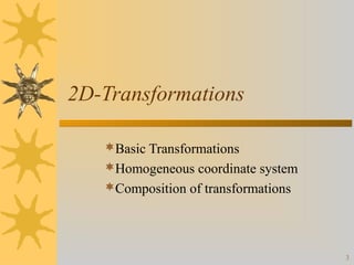
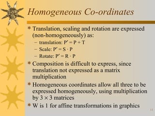
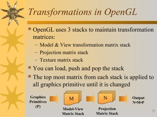
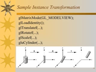
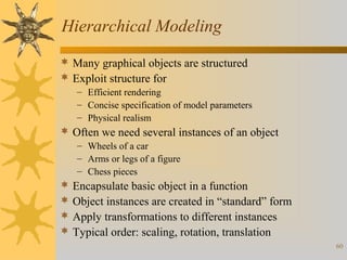
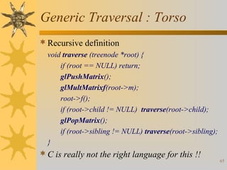
![Vectors in 3D
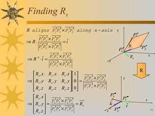
Have length and direction
V = [xv , yv , zv]
Length is given by the Euclidean Norm
||V|| = √( xv2 + yv2 + zv2 )
Dot Product
V • U = [xv, yv, zv]•[xu, yu, zu]
= xv*xu + yv*yu + zv*zu
= ||V|| || U|| cos ß
Cross Product
V×U
= [yv*zu - zv yu , -xv*zu + zv*xu , xv*yu – yv*xu ]
= η ||V|| || U|| sin ß
V × U = - ( U x V)
z
K
J+c
b
aI+
V=
(xv,yv,zv)
y
x
23](https://image.slidesharecdn.com/modelingtransformations-131112131436-phpapp02/85/Modeling-Transformations-23-320.jpg)
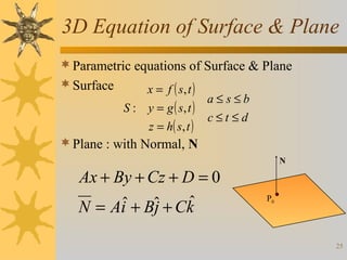
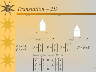
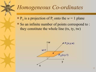
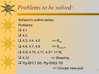
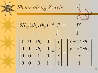
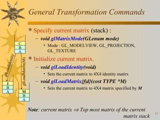
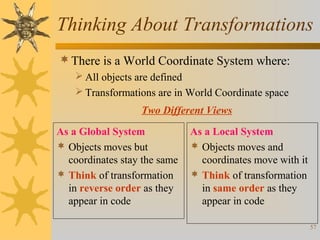
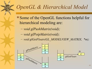
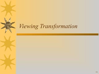
![3D Plane
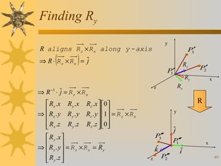
Ways of defining a plane
1. 3 points P0, P1, P2 on the plane
2. Plane Normal N & P0 on plane
3. Plane Normal N & a vector V on the plane
N
Plane Passing through P0, P1, P2
ˆ
ˆ
N = P0 P × P0 P2 = Ai + Bˆ + Ck
j
1
P0
if P(x, y, z) is on the plane
N • P0 P = 0
[
P1
P2
V
]
ˆ
ˆ
ˆ
ˆ
⇒ ( Ai + Bˆ + Ck ) • ( x − x0 )i + ( y − y0 ) ˆ + ( z − z0 )k = 0
j
j
⇒ Ax + By + Cz + D = 0
where D = −( Ax0 + By0 + Cz0 )
26](https://image.slidesharecdn.com/modelingtransformations-131112131436-phpapp02/85/Modeling-Transformations-26-320.jpg)
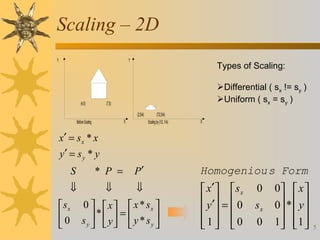
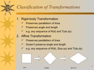
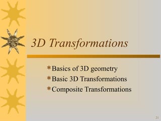
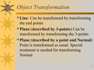
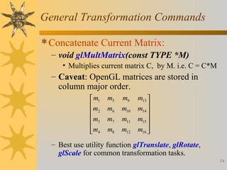
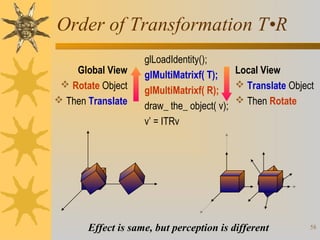
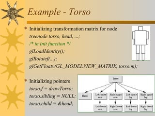
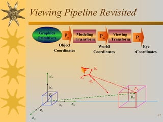
![Affine Transformation
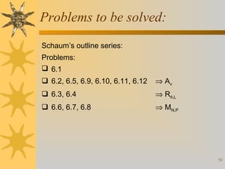
Transformation – is a function that takes a point (or vector) and
maps that point (or vector) into another point (or vector).
A coordinate transformation of the form:
x’ = axx x + axy y + axz z + bx ,
y’ = ayx x + ayy y + ayz z + by ,
z’ = azx x + azy y + azz z + bz ,
x' a xx
y ' a yx
z' = a
zx
w 0
a xy
a xz
a yy
a zy
a yz
a zz
0
0
bx x
b y y
bz z
1 1
is called a 3D affine transformation.
The 4th row for affine transformation is always [0 0 0 1].
Properties of affine transformation:
– translation, scaling, shearing, rotation (or any combination of them) are
examples affine transformations.
– Lines and planes are preserved.
– parallelism of lines and planes are also preserved, but not angles and
length.
27](https://image.slidesharecdn.com/modelingtransformations-131112131436-phpapp02/85/Modeling-Transformations-27-320.jpg)

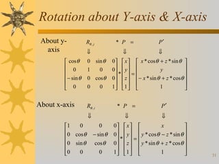
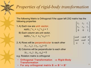
![Finding Rz
R aligns P1′P2′ along z - axis
⇒ R⋅
P1′P2′
P1′P2′
P′
3
ˆ
=k
ˆ = P1′P2′
⇒ R ⋅k
P1′P2′
T
Rx . x
⇒ Rx . y
Rx .z
y
R y .x
Ry . y
R y .z
Rz
[ R
−1
=R
T
P′
1
]
x
z
R
Rz . x 0
P ′P ′
R z . y 0 = 1 2
′ ′
Rz .z 1 P1P2
Rz . x
R . y = P1′P2′ = R
⇒ z
z
Rz .z P1′P2′
P2′
y
′
P′
3
ˆ
k
z
′
P2′
′
P′
1
x
47](https://image.slidesharecdn.com/modelingtransformations-131112131436-phpapp02/85/Modeling-Transformations-47-320.jpg)
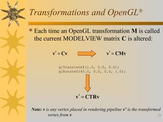
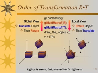
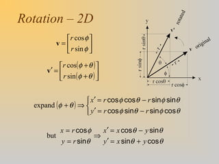
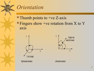
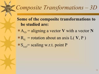
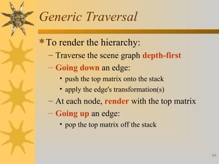
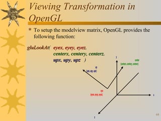
![Scene Graph
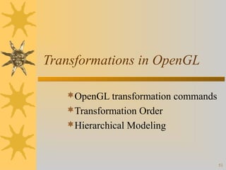
A scene graph is a hierarchical representation of a scene
We will use trees for representing hierarchical objects
such that:
– Nodes represent parts of an object
– Topology is maintained using parent-child relationship
– Edges represent transformations that applies to a part and all the
subparts connected to that part
Scene
typedef struct treenode {
GLfloat m[16]; // Transformation
Sun
Star X
void (*f) ( );
// Draw function
struct treenode *sibling;
Earth
Venus
Saturn
struct treenode *child;
} treenode;
Moon
Ring
62](https://image.slidesharecdn.com/modelingtransformations-131112131436-phpapp02/85/Modeling-Transformations-62-320.jpg)


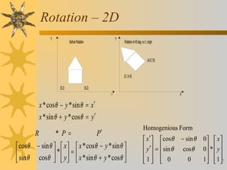
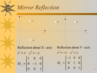
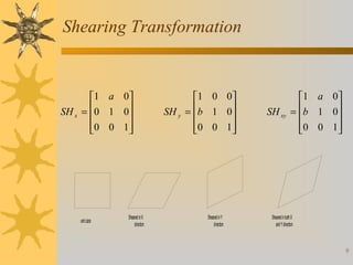
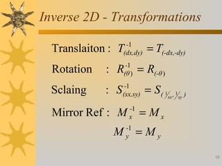
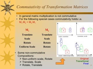
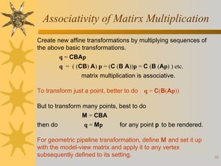
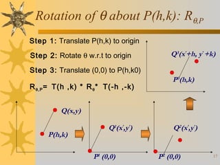
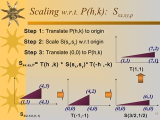
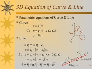
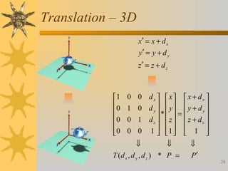
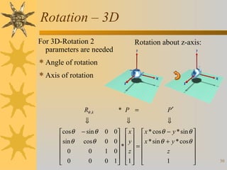
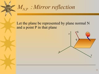
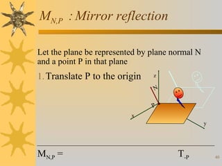
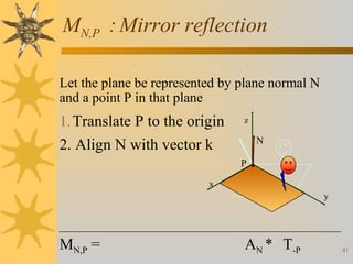
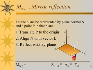
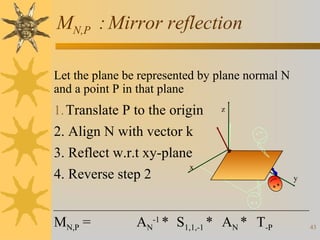
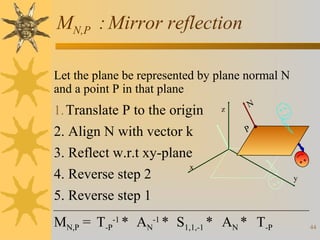
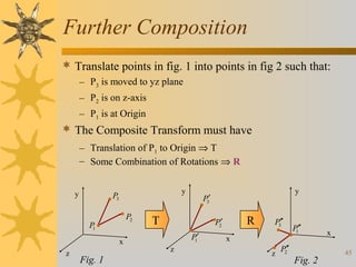
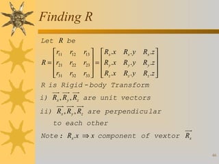
The document discusses various 2D and 3D transformations including translation, scaling, rotation, reflection, shearing, and homogeneous coordinates. It provides the mathematical definitions and matrix representations for each transformation type in 2D and 3D. It also covers topics like composition and inverse of transformations, classification of transformations, and properties of rigid body transformations.