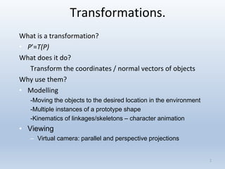
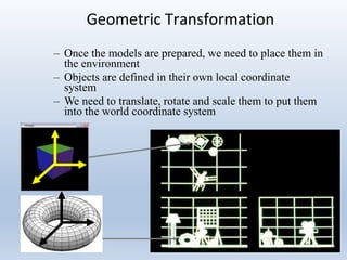
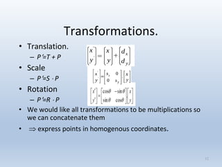
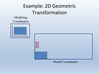
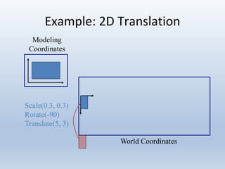
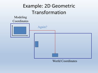
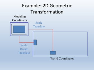
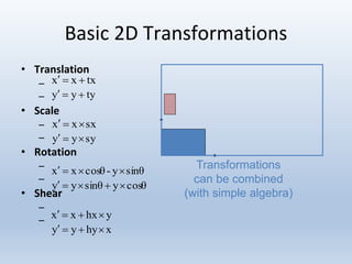
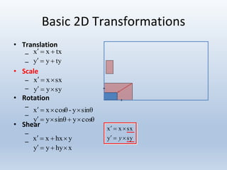
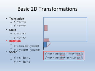
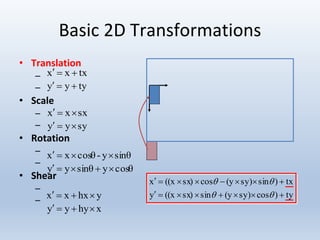
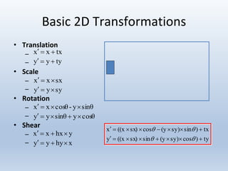
Transformations are used to move and manipulate 3D objects in computer graphics. The key types of 2D transformations are:
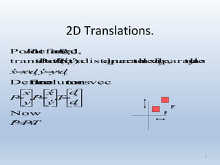
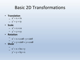
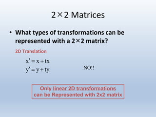
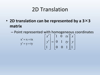
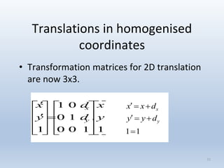
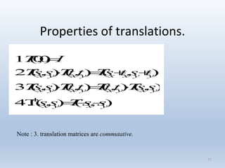
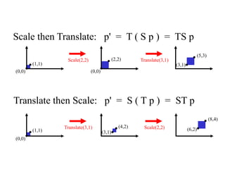
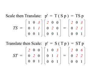
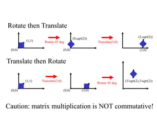
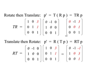
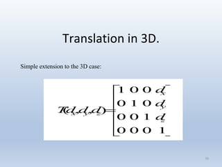
1. Translation moves objects by adding offsets to the x and y coordinates.
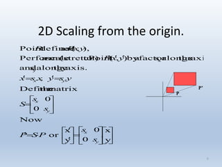
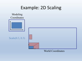
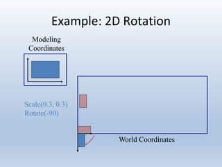
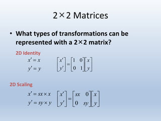
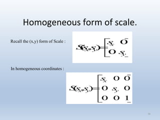
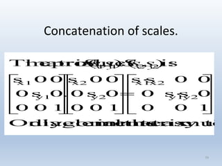
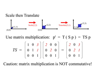
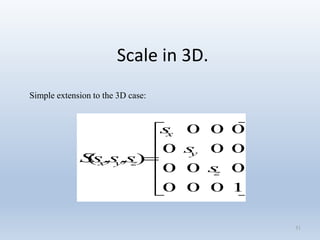
2. Scaling enlarges or shrinks objects by multiplying the x and y coordinates by scale factors.
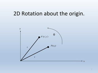
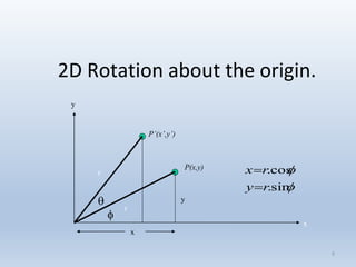
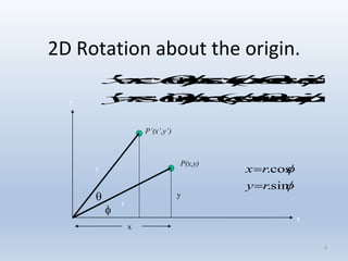
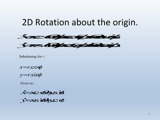
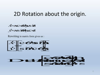
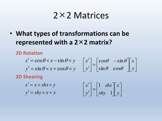
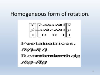
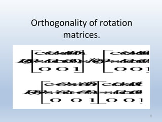
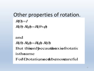
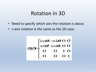
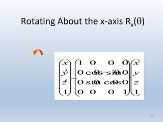
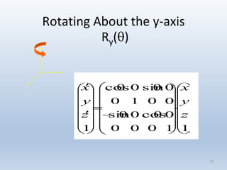
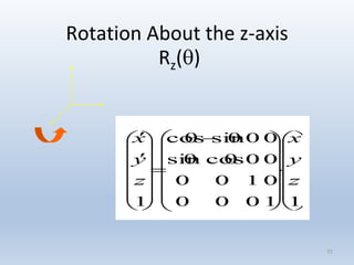
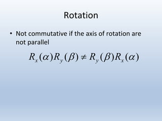
3. Rotation spins objects around the origin by applying trigonometric functions to the coordinates.
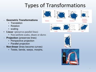
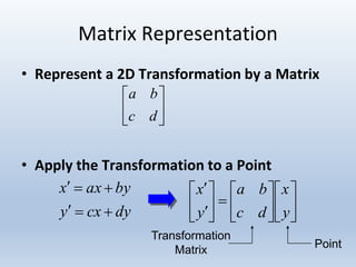
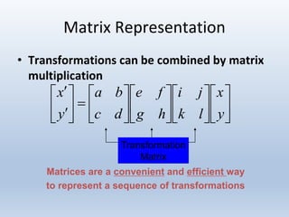
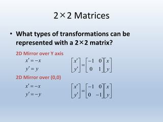
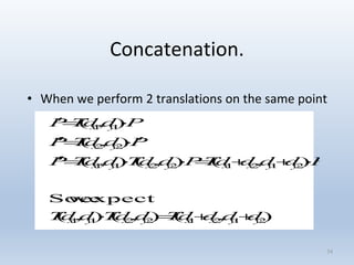
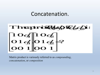
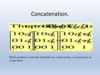
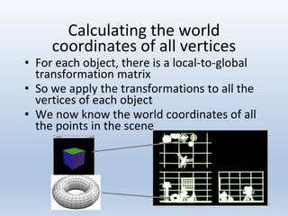
Transformations can be represented using matrices, allowing multiple transformations to be combined through matrix multiplication. Common 2D transformations like translation, scaling, rotation, and shearing can be encoded concisely using 2×2 transformation matrices.